Easy log rank test for survival analysis

Previously, we talked about survival analysis and the Kaplan-Meier curve. In this post, I will explain how to interpret the log rank test for survival analysis.

Before we start, you might want to check out my previous blogposts for an easy introduction to survival analysis and the Kaplan-Meier curves. As you’ve probably guessed from the title, we use the log rank test to evaluate differences between survival curves… but there’s a bit more to it!

In this post, we will discuss the main concepts behind the log rank test – easily explained!

So if you are ready… let’s dive in!

What is the log rank test?

Sometimes, it is very obvious to the eye that two survival curves are very similar, or very different. But we need an objective way to quantify the differences between two survival curves, and we do that with the log rank test.

The log rank test is the most common method to quantify differences between two survival groups. This test compares the distribution of the time until an event occurs of two or more independent samples.

Log rank test – easily explained with an example!

As we mentioned before, the log rank test can be used to test whether there is a difference between two or more groups. In particular, we test whether there is a difference in the time it takes for an event to occur.

Remember that in survival analysis, we look at a variable that has a start time and an end time, which is when a certain event occurs. An event can be the death of patient, but also taking your cast off after breaking your arm, or finishing a 5k run!

Let’s focus on the classical example in a clinical trial setting. We want to test whether drug A is better than drug B, whether it increases survival time of the patients.

Our start time is the day the patient got the first dose of drug A or B.

Our event of interest is death. We are interested in the time between the start and the end.

And our two groups are patients that were given drug A versus patients that were given drug B. Note that we could be comparing survival between men and women, or between patients with and without a particular risk factor (for example, smokers and non-smokers, patients with BRCA1 mutation versus patients without it…).

We collect data from different patients over 5 years and plot a Kaplan-Meier curve. In this case, the curves are slightly divergent. It looks like drug A improves the survival time of patients. If we check the curve at 50%, the median survival time is slightly higher in group A versus group B.

But is the difference between them significant? For this we need the log rank test.

Hypotheses in the log rank test

The null hypothesis is that both groups have identical distribution curves.

The alternative hypothesis is that both groups have different distribution curves.

In summary, we are testing whether the survival curves are identical (overlapping) or not.

Of course, the maths are bit more complicated than that, but this way you can get an intuitive understanding of the log rank test.

How to interpret log rank test results

As with any statistical tests, the log rank test will give us a p-value. Depending on the threshold we use, for example, 0.05:

p-val <0.05: we reject the null hypothesis, in other words, there is a significant difference between two groups. In our example, drug A significantly improves the survival compared to drug B

p-val > 0.05: with this data, we cannot reject the null hypothesis. This means that the two curves are not statistically significantly different. With this data, we cannot say if there is a significant difference between the two groups. Careful! There could be differences between drug A and drug B. For example, you might have a very small dataset, so you don’t have enough statistical power to rule out a real difference and avoid a type two error (false negative).

How is the log rank test calculated?

If you would like to understand the maths behind the log rank test, I can recommend you this webpage. You will find a beautiful explanation of the calculations behind the log rank test, step-by-step with an example.

Here, I will just give you a few notes to get an intuitive understanding of how the log rank test is calculated.

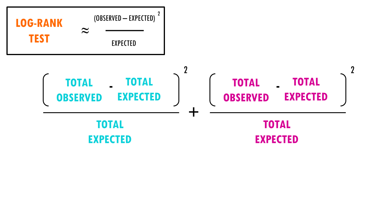
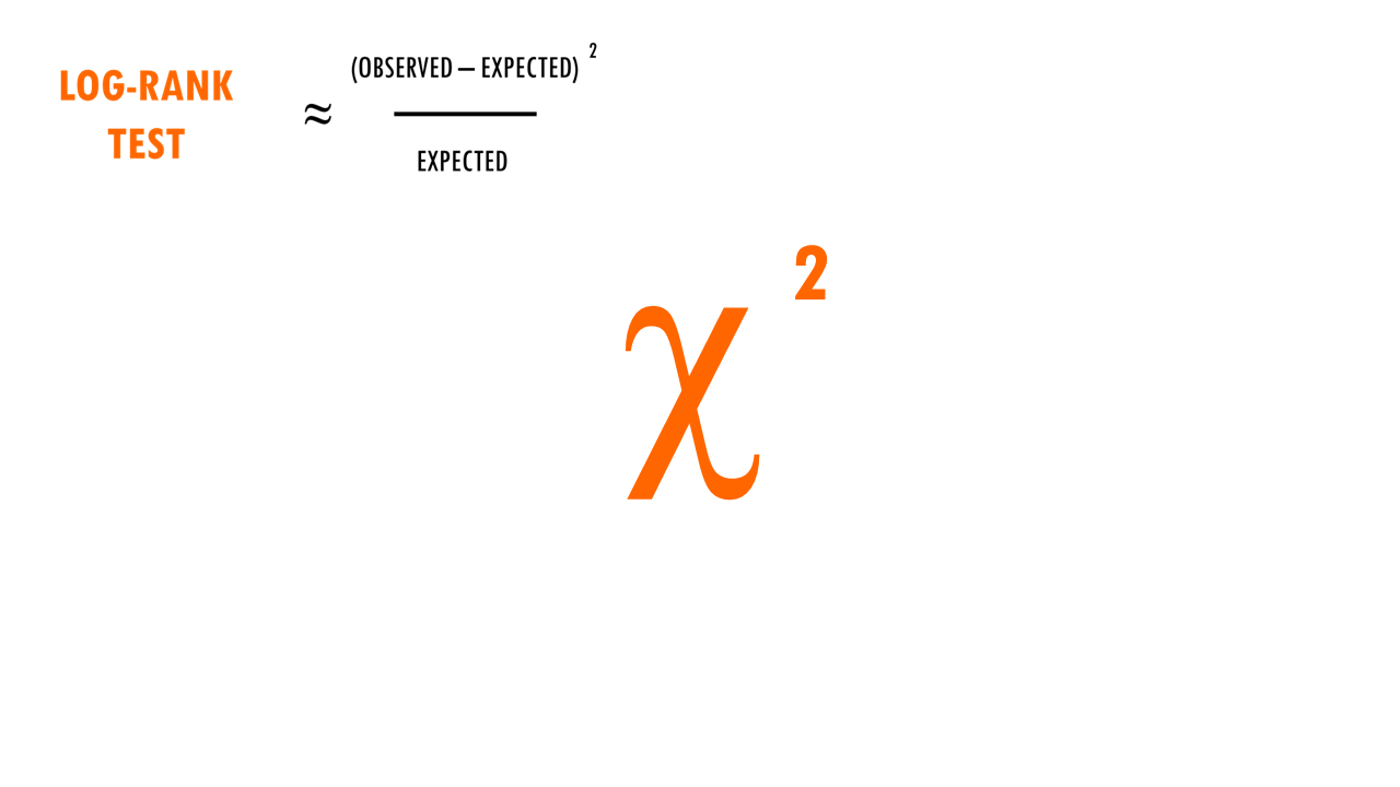
In essence, the log rank test is a chi-square (X²) test. 

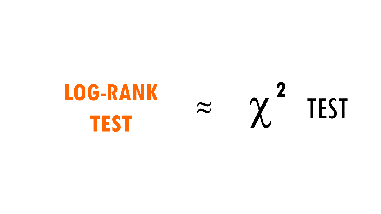
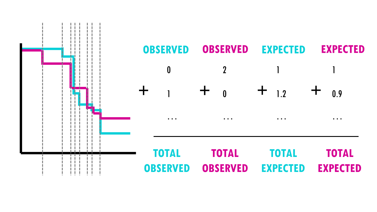
For each group, we compute a chi-square test on the sum up the observed and expected events at each time interval, and then sum up the results.

Wait a minute. Let’s take that bit by bit.

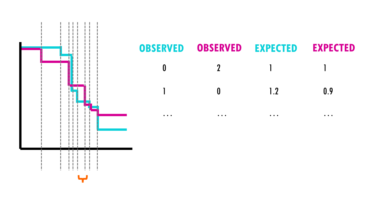
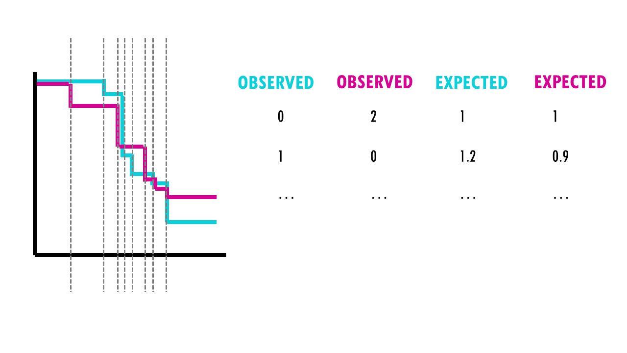
Going back to our example, for each group, the log rank test will do a big calculation. For example, for patients who were given drug A, it does some maths. Then, it does some maths with data from patients who were given drug B.

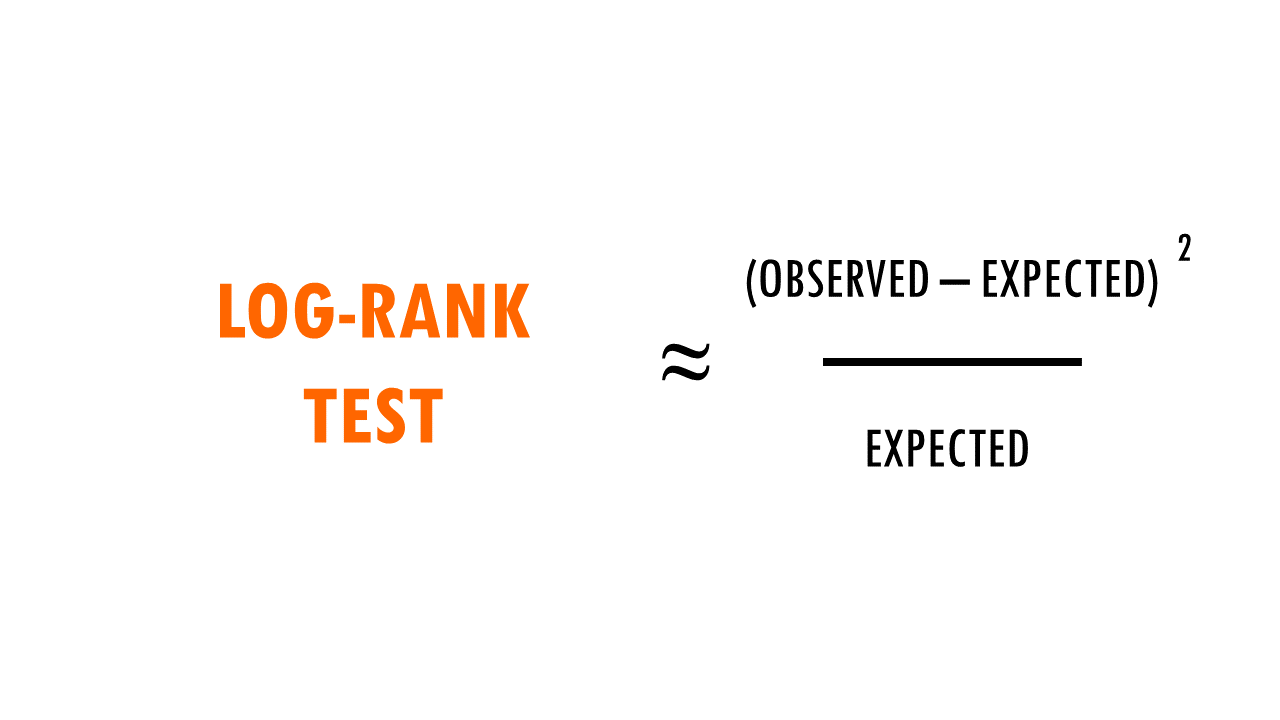
So what are these mysterious maths? Well, it’s an easy chi-square test! The log rank test calculates the X2 test statistic. This statistic compares the observed number of events (deaths) versus the expected number of events (more about how to calculate what is ‘expected’ later on).

But it does that for each event time (e.g., in this example, it would be 12 months, then 15 months, then 17 months…). We then sum the total number of observed and expected numbers of events in each group over time.

Finally, the summed results for each group (in this case, drug A and drug B), are used to calculate the ultimate chi-square statistic.

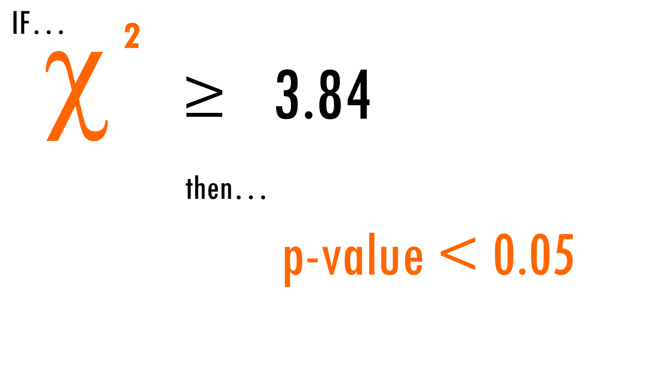
We can then use this X2 statistic to decide whether the curves are statistically different or not. If we have a look at the X2 distribution table, and figure out that for a significance level of 0.05, and 1 degree of freedom, we can reject the null hypothesis if X2 > 3.84. Since X2 = 7.2 in our example, we can reject the null hypothesis: we have significant evidence (alpha = 0.05) that the two survival curves are statistically different.

Easy!

‘Expected number of events’?

We mentioned the expected number of events before. But how can we know that the is the expected number of deaths in patients who were given drug A?

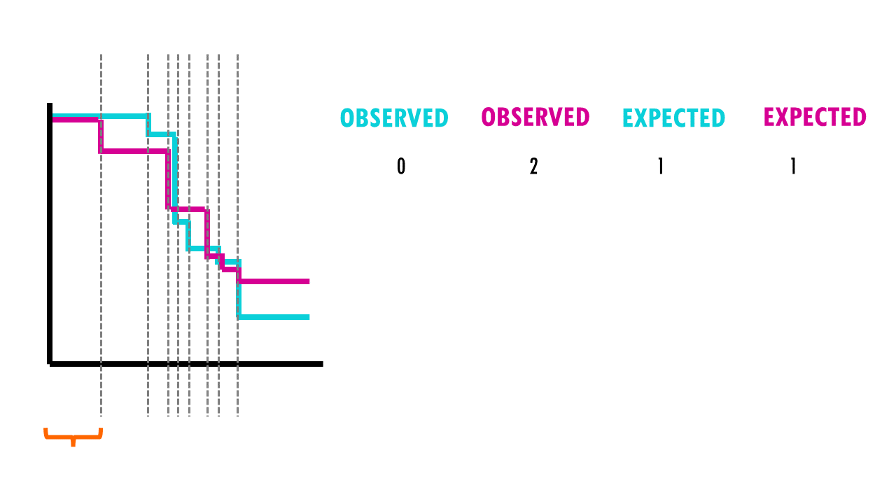
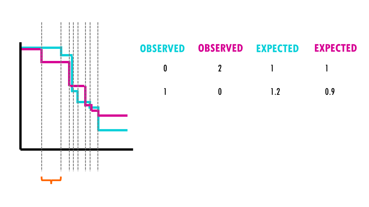
First, you must know that the expected number of events assumes that the null hypothesis is true and the survival groups are identical. To generate the expected number of events we basically take data from both groups combined and estimate the proportion of events that occur at that time interval, regardless of the group in which the event occurred.

For example, we have 50 patients, 30 in the first group (drug A) and 20 in the second group (drug B). During the first week, 2 patients in the first group died, and no patient from the second group died. At the start of the week, there were 50 patients alive in total, so the risk of death in this week was 2/50. 

• There were 30 patients in group 1, so, if the null hypothesis were true, the expected number of deaths in group 1 is 30× 2/50 = 1.2.
• In group 2 the expected number of deaths is 20× 1/50 = 0.8.

Is the log rank test enough?

In summary, the log rank test is used to test whether there is a difference between the survival times of different groups. However, it does not provide an estimate of the size of the difference between the groups or a confidence interval.

Moreover, with the log rank test, we might compare the survival of a group of patients who received drug A, versus the survival times of patients who received drug B.

But what about including their age? Or gender? Or presence of a certain mutation? The log rank test does not allow other explanatory variables to be taken into account.

That is when we need Cox Proportional Hazards Survival Regression.

Want to know more?

If you would like to know more about common survival time analysis, check out:

• Survival analysis basics R tutorial.

You might be interested in…

• Survival time analysis: easily explained!
• Kaplan-Meier curves easily explained

• If you want to know more about X2 tests, check out my blogpost on Chi-square, easily explained!
• If you are interested in learning how to calculate the log rank test manually, check out this website!
• This other website has an exhaustive step-by-step workflow of computing the log rank test with an example.

Ending notes

Wohoo! You made it ’til the end!

In this post, I shared some insights on survival time analysis.

Hopefully you found some of my notes and resources useful! Don’t hesitate to leave a comment if there is anything unclear, that you would like explained differently/ further, or if you’re looking for more resources on biostatistics! Your feedback is really appreciated and it helps me create more useful content:)

Before you go, you might want to check:

Squids don't care much for coffee,

but Laura loves a hot cup in the morning!

If you like my content, you might consider buying me a coffee.

You can also leave a comment or a 'like' in my posts or Youtube channel, knowing that they're helpful really motivates me to keep going:)

Cheers and have a 'squidtastic' day!