ANOVA (analysis of variance) easily explained

When you’re working with data and want to determine whether different groups have significantly different averages, simply eyeballing the numbers won’t cut it. That’s where ANOVA (Analysis of Variance) comes in.

ANOVA is a statistical method used to compare the means of three or more groups to see if at least one is significantly different from the others. It’s widely used in fields like psychology, medicine, marketing, and beyond—anywhere researchers need to test hypotheses across multiple conditions. In this post, we’ll break down what ANOVA is, when to use it, how it works, and what its results really tell you.

So if you’re ready… let’s dive in!

When do we need ANOVA?

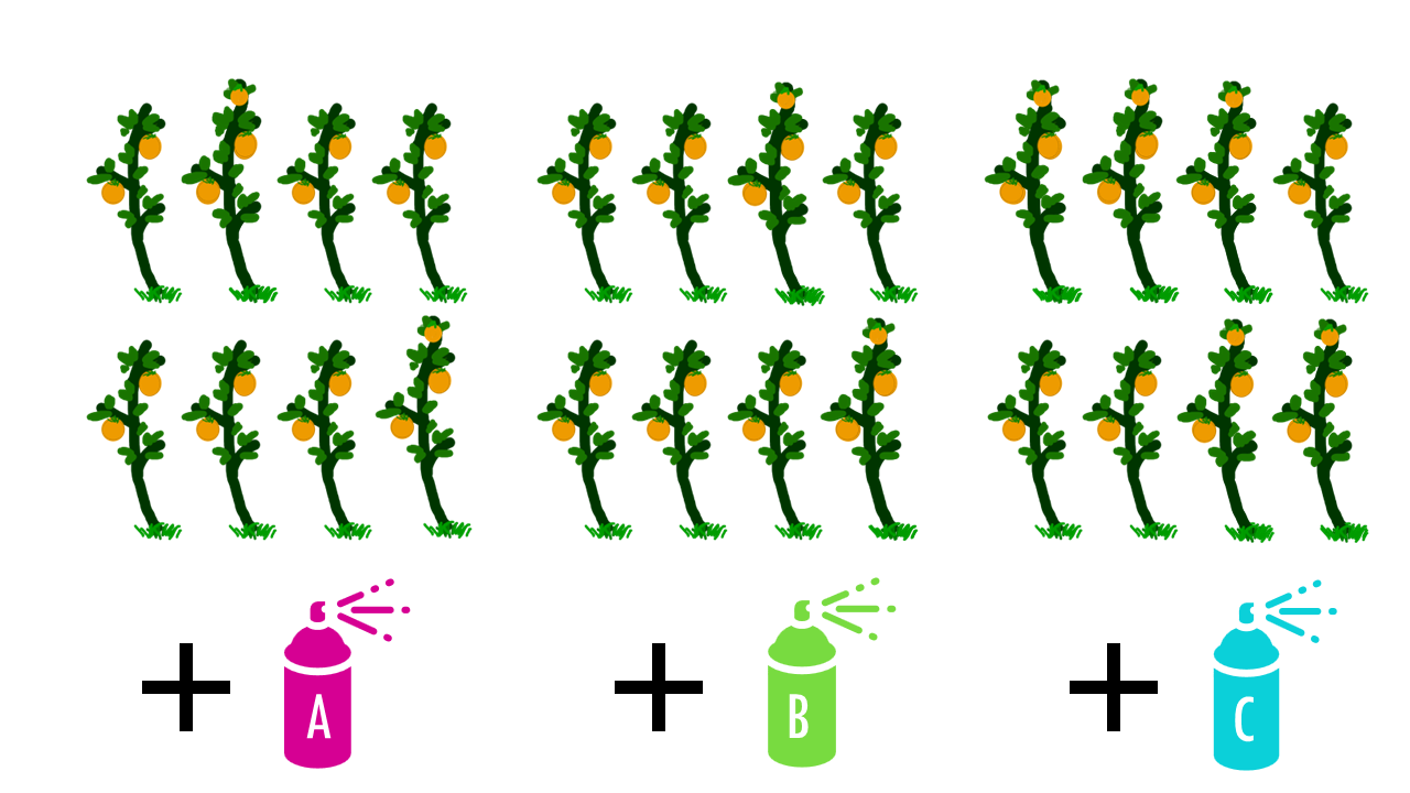
Let’s imagine you’ve just invented three new super-fertilizers: Fertilizer A, B, and C. — and you want to know: which one makes plants grow the tallest?“

Each group of plants gets a different fertilizer, and after four weeks, you measure their height.

Now it’s time to check if the difference in plant height between groups is real, if it’s statistically significant – in other words, if one of the fertilisers actually works better than the others.

If we wanted to compare fertilisers A and B, we could use a standard t-test to compare their means. However, when we have more than 2 groups, we would need to make pairwise comparisons between each combination of the groups and using multiple t-tests increases the risk of Type I error (false positives). So the probability of concluding that there is a difference between fertilisers – when in fact there isn’t – increases.

That is why when we want to compare more than two groups we use analysis of variance or ANOVA, which controls for false positives by testing all groups simultaneously.

One-way ANOVA

ANOVA (Analysis of Variance) is a statistical method used to test whether there are significant differences between the means of three or more independent groups. For example, evaluating different treatments or conditions like

• Different drug treatments
• Different environmental conditions (temperature, pH, light, etc.)
• Different species or strains

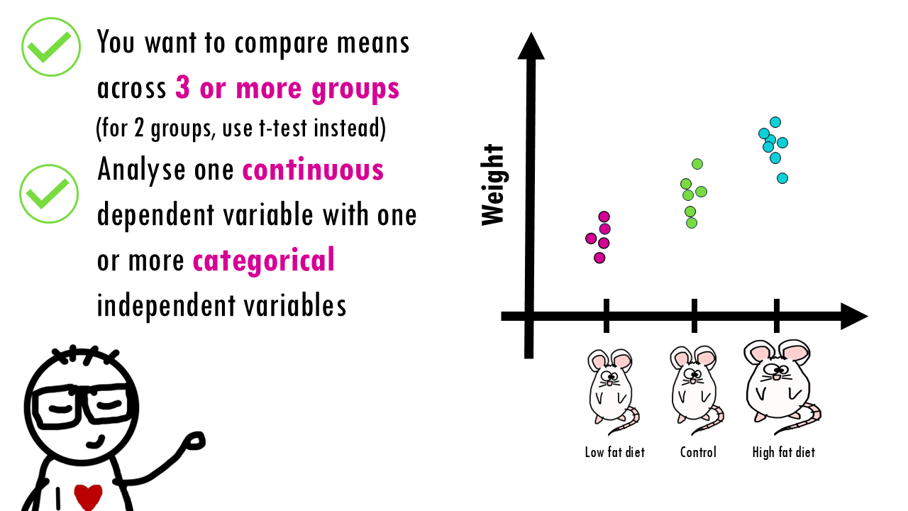
So, our question is, do these fertilizers make a statistically significant difference in plant growth, or is it just random chance that one group grew more than the other?

Let’s break down ANOVA in 4 simple steps.

Step 1: Hypotheses of ANOVA

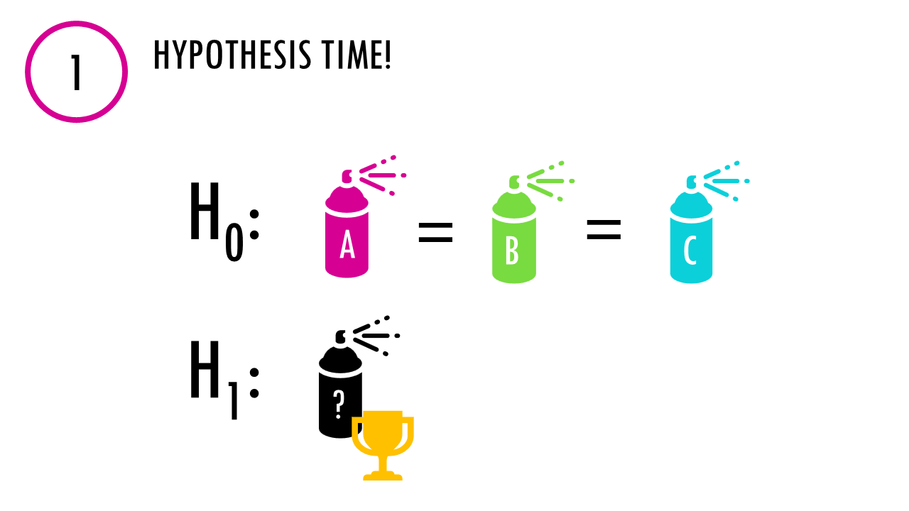
Step 1: Hypotheses Time! As with any hypothesis test, we state our null and alternative hypotheses.

• Null Hypothesis (H₀): “All fertilizers are equal. No difference in plant height.”

• Alternative Hypothesis (H₁): “At least one fertilizer is doing magic – there are differences in the average height of plants between groups”

The test will give us a p-value, and if it is low enough, we can say that there is a statistically significant difference between at least one fertiliser.

Step 2: Calculating variability

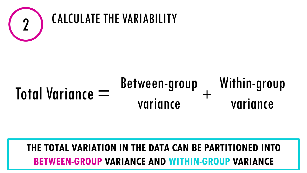
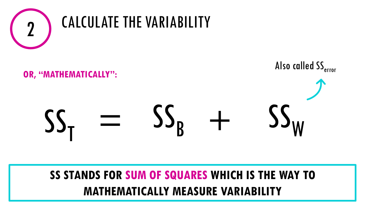
The core idea is to partition the total variation in your data into two components. ANOVA looks at two kinds of variation:

1. Between-Groups Variance (SSB): Measures how group means differ from the overall mean.
   “Are the group averages far apart?”
2. Within-Groups Variance (SSW or SSerror): Measures how individual values vary within each group.
   This is also called the error variance. Even if all plants within a group were given the same fertiliser, there’s going to be some variability. When comparing groups we need to take into account this within-groups variance, which contains all the unexplained variance – variance that is not due to the fertilisers.

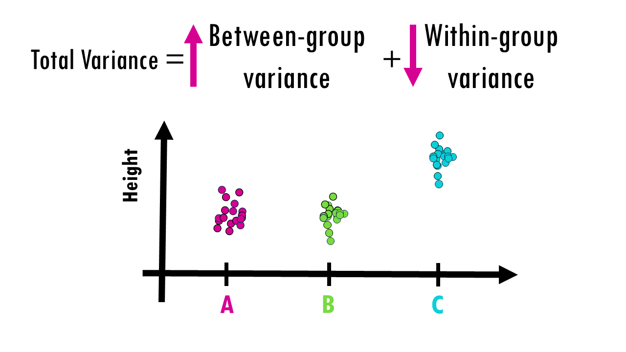
Let’s just visualise this with a few examples. Imagine the measurements of height between groups look like this. It’s easy to say fertiliser C is much better right? The variance within groups is very small, but the variance between groups – in this case between C and the other groups – is quite big.

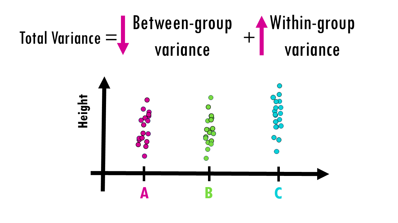
Now imagine the measurements of height look like this. It’s not so clear now. C has a slightly higher average, but the variance within each group is quite big, and the variance between groups is not that big – in actual fact, it could be just noise and just by random sampling you picked the highest plants that were given fertiliser C, and smaller plants that got fertilisers A and B. If you repeated the experiment again, A or B could be slightly higher.

So essentially, ANOVA quantifies this, giving us a number that will help us decide whether there is or not a difference between at least one of the groups. If at least one of the groups truly has a different mean, the between-group variation should be large relative to the within-group variation.

The value I’m referring to is the F-value.

F = (Between-group variance) / (Within-group variance)

More specifically:

• Between-group variance (MSB): Mean sum of squares between groups
• Within-group variance (MSW): Mean sum of squares within groups (error variance)

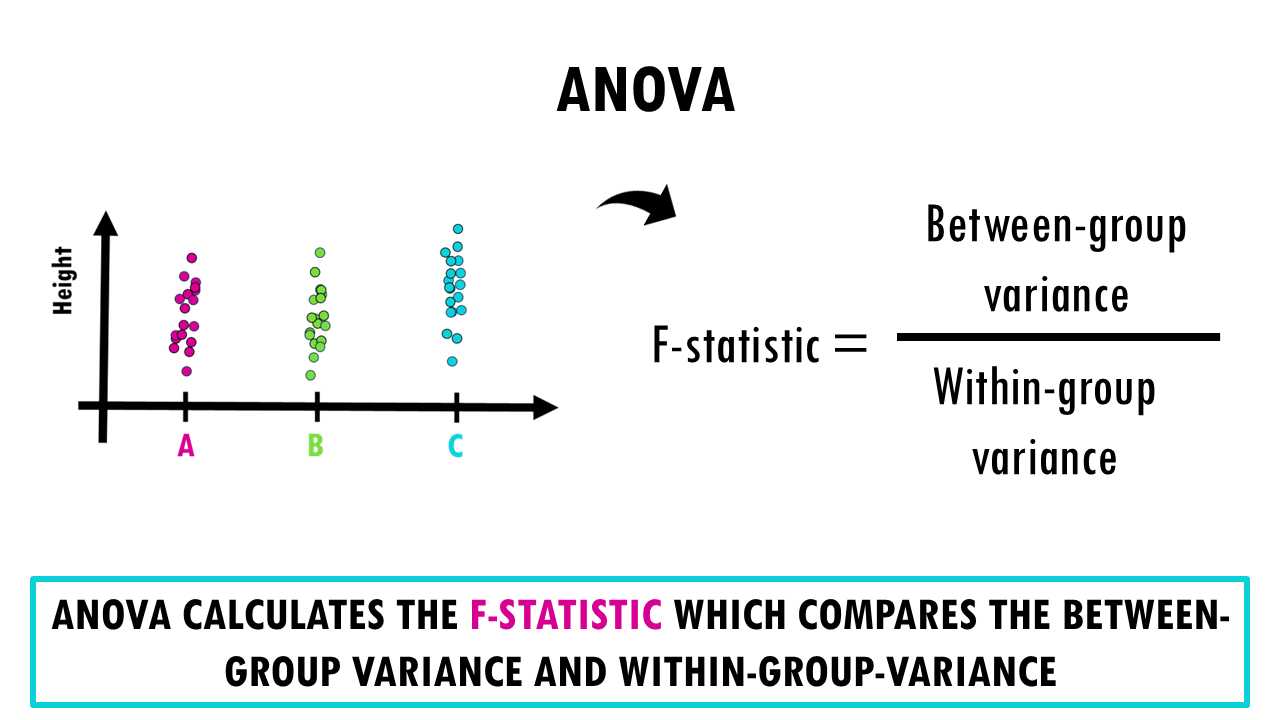
Essentially, we’re testing whether the between-group variance is significantly larger than the error variance.

Wait a minute! How did we get MS values from SS values?! The SS values represent the actual partitioning of total variance into components. The Mean Sum of Squares or mean squares are actually the SS values divided by their degrees of freedom. This gives us an unbiased estimate of the different variance components, or the different sources of variation. Raw SS values depend on sample size – larger samples naturally have larger SS values even with the same underlying variance. Dividing by degrees of freedom adjusts for this, giving us variance estimates that can be fairly compared regardless of sample size.

So, to summarise, we use the MS values to calculate F-statistics because they’re proper variance estimates.

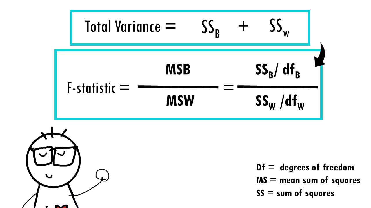
Back to our F value. You want your F value to be big (>1)– that is, your small variance within groups, but big variance between groups. A smaller F value (close to 1) means the group means are likely similar (null hypothesis not rejected).

Step 3: Get the ANOVA p-value

With the ANOVA test, as with any statistical test, we get a p-value. As we know, with every statistical test comes uncertainty. The p-value tells you the probability of observing an F-statistic as large as (or larger than) the one you calculated, assuming the null hypothesis is true.

In other words, if all group means are equal (so no differences between fertilisers), (in this example) there’s a 1.2 % chance you’re seeing these differences between fertilisers.

It’s up to you to decide on the level of significance, but a

• Small p-value (typically < 0.05): Strong evidence against the null hypothesis, suggesting at least one group mean differs significantly. There is a statistically significant difference in plant height among fertilizers.
• Large p-value: Insufficient evidence to conclude that group means differ. With this data we cannot say there is a difference in height (but maybe we just need a bigger sample!! We cannot claim that there is no difference!)

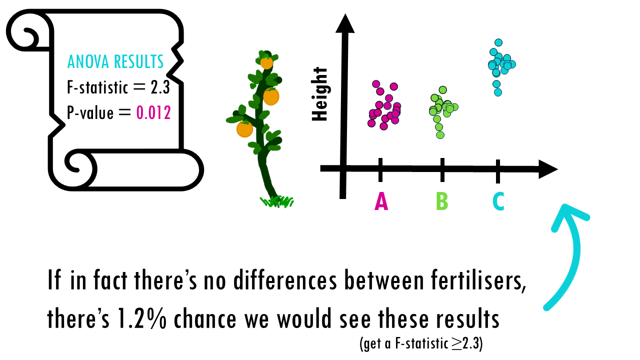
We got a p-value of 0.012 which is lower than 0.05, we can say that there is a difference! At least one fertilizer had a different effect in plant height than the rest! But wait… we still don’t know which one!

Step 4: Post-hoc test

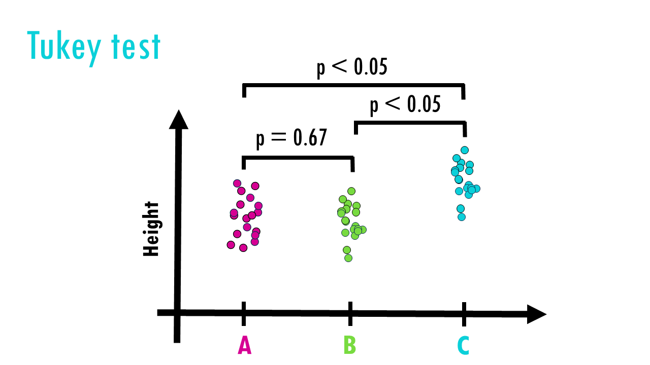
We often use a post-hoc test like a Tukey test to make pairwise comparisons and decide which fertilisers are different between each other:

• A vs B?
• A vs C?
• B vs C?

Tukey’s test a better option for multiple pairwise comparisons than a Student’s t-test because of several reasons:

• Controls for family-wise error rate across all pairwise comparisons.
• Adjusts p-values so the overall risk of Type I error stays at 5%.
• Works well when sample sizes are equal (or nearly so).
• Designed specifically as a post-ANOVA tool for all pairwise group comparisons.

You might wonder, “If I really just want to know which groups differ, why not skip ANOVA and jump straight to the Tukey test?”. The short answer is that Tukey’s test assumes you’ve already found a significant result using ANOVA. It’s designed to control the error rate after you’ve found a significant difference somewhere.

Great! So Tukey’s test tells us Fertilizer C is the winner! It made plants grow significantly taller than A and B.

Two-way ANOVA

But wait! We forgot to take into account sunlight conditions!! Now you’re testing TWO independent variables at the same time — and maybe how they interact. So now we have two variables:

• Fertilizer Type (A, B, C)
• Sunlight Level (Low, High)

The question now is, “Does fertilizer type, sunlight level, or their combination affect plant height?”

If we break it down, there’s actually three different different questions here:

1. Does fertilizer affect growth?
2. Does sunlight affect growth?
3. Is there an interaction effect? (e.g. maybe Fertilizer A only works in high sun)

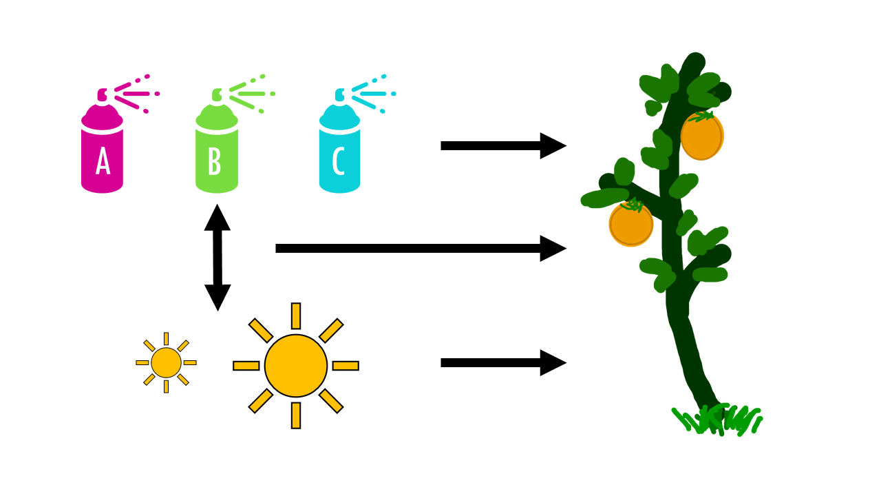
One way ANOVA isn’t enough here… we need two-way ANOVA. Two-way just means we’re testing two factors – actually, we’re testing each factor — fertilizer AND sunlight — but also whether their combination has a special effect.

Like with one-way ANOVA, we split the total variation we observe between plant heights into groups.

Two-way ANOVA partitions the total variation into four components:

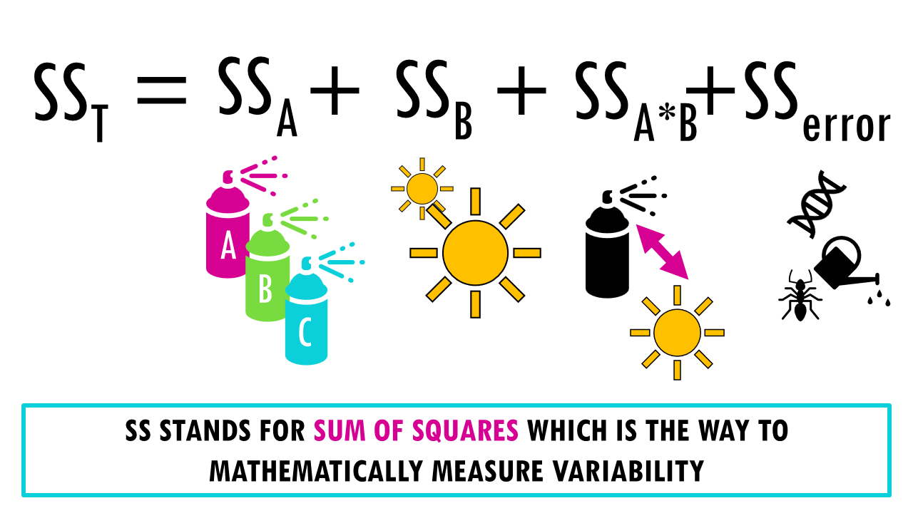
Total variation = SS_A + SS_B + SS_AxB + SS_error

1. Main effect of Factor A: how much of the total variation in height is due to differences between fertilizer types?
2. Main effect of Factor B: How much sunlight levels alone affect plant height
3. Interaction effect (A × B): How the combination of factors affects the outcome beyond their individual effects
4. Error/residual variation: Unexplained variation within groups. What’s left over — random variation between individual plants.

Two-way ANOVA produces three separate F-tests: one for the type of fertiliser, one for sunlight and one for the interaction. We get the F statistic exactly the same way, first dividing each sum of squares by its degrees of freedom to get the mean square values, then dividing each source of possible between-group variation by the within-group variation or the error variation:

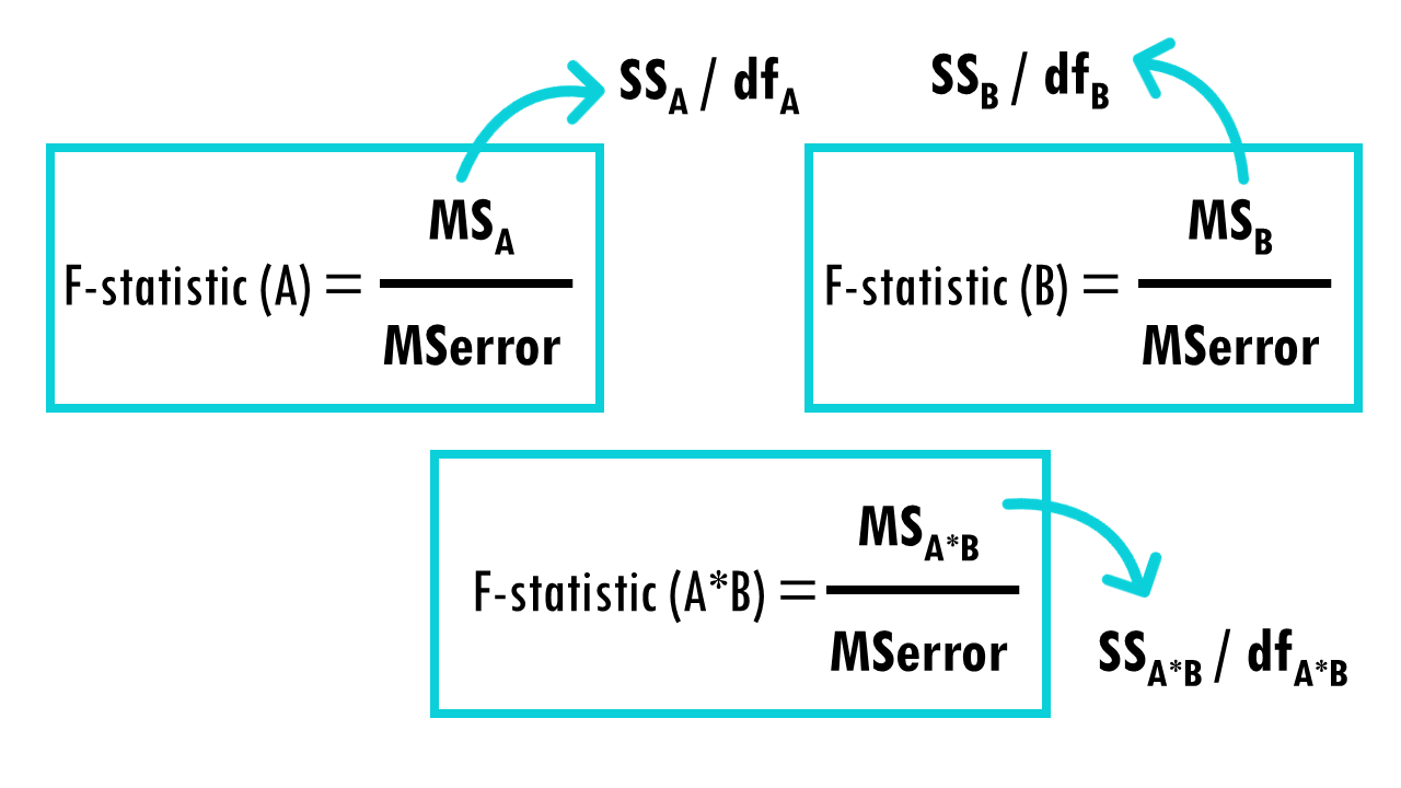
Each F-statistic gets its own p-value, so you’re testing three hypotheses simultaneously. And each of the p-values tells you whether that source of variance is statistically significant.

Interpreting two-way ANOVA results

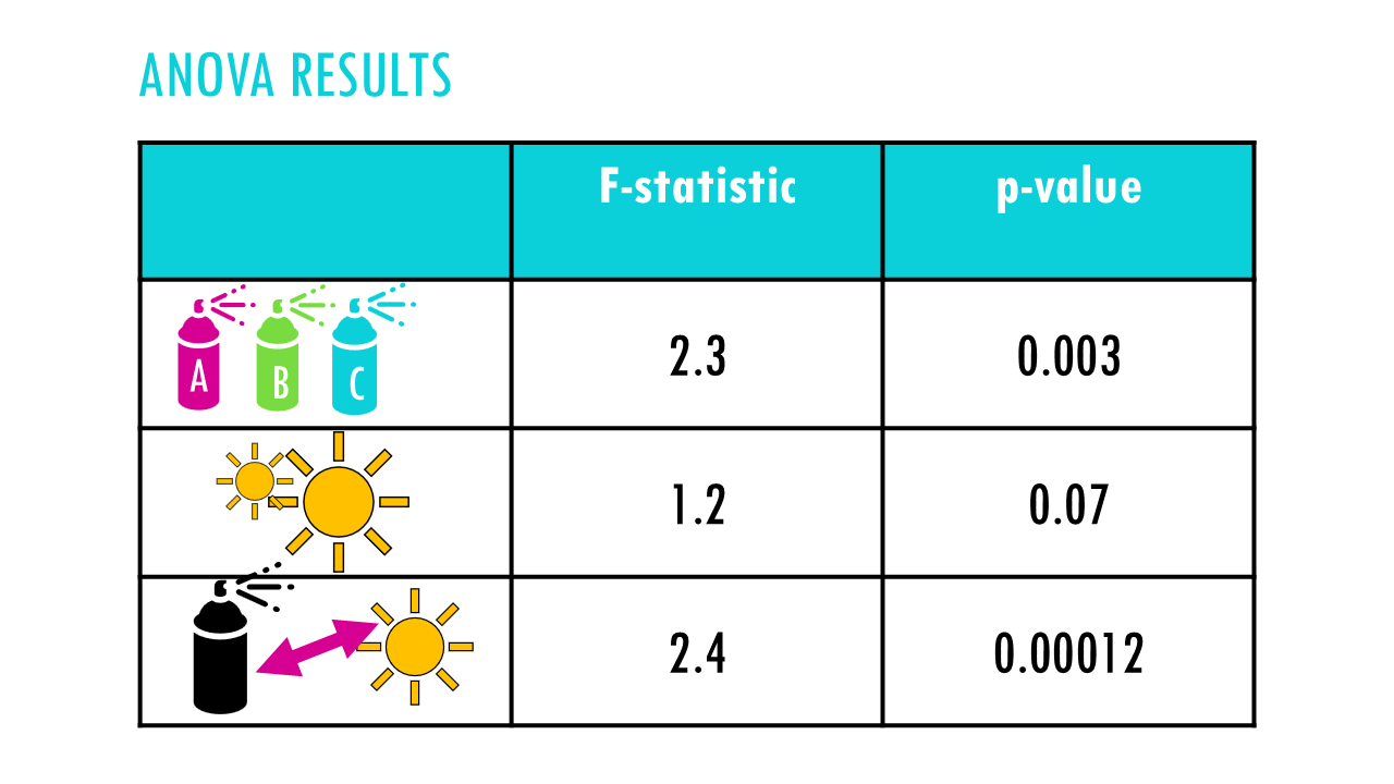
How do you interpret the results of two-way ANOVA? If there’s a significant interaction, you typically focus on that rather than the main effects, since the main effects can be misleading when an interaction is present.

For example, in this case, it looks like there is an interaction between the fertilisers and sunlight.

The main effects we saw previously with fertiliser C become less meaningful because the effect of fertilisers depend on sunlight levels. We might find that fertiliser C works best with sunlight, and fertilisers B works best with less light. We would need to examine the interaction plot and do simple effects analysis.

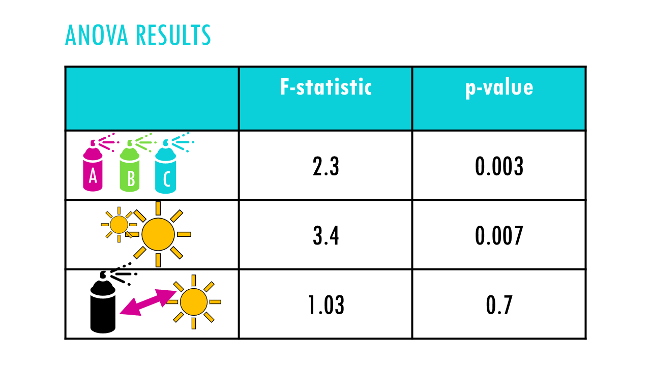
In this other example, it looks like at least one fertiliser works better overall, and sunlight levels also matter. However there doesn’t seem to be an interaction between both – the effect of sunlight is consistent across all three fertilisers.

When to use ANOVA? ANOVA assumptions

Nice! So to recap, ANOVA (Analysis of Variance) is a statistical method used to test whether there are significant differences between the means of three or more independent groups. For example, evaluating different treatments or conditions like

• Different drug treatments
• Different environmental conditions (temperature, pH, light, etc.)
• Different species or strains

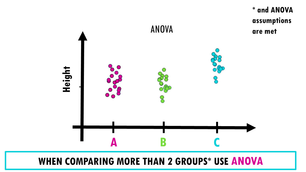
To use ANOVA correctly, you need to make sure your data meets ANOVA’s assumptions:

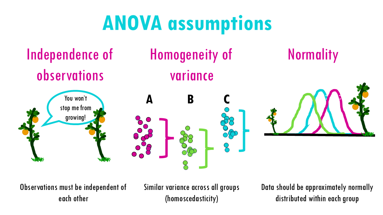
• Independence of Observations: The observations within each group should be independent of each other. In this case, each plant’s height is independent and does not influence the height of other plants.
• Homogeneity: The variances in each group should be roughly the same. This can be checked with the Levene test. If the condition of variance homogeneity is not fulfilled, Welch’s ANOVA can be calculated instead of the “normal” ANOVA. 
• Normal distribution: The data within the groups should be normally distributed. This means that the majority of the values ​​are in the average range, while very few values ​​are significantly below or significantly above. If this condition is not met, the Kruskal-Wallis test can be used.

Final notes

In summary, both one-way and two-way ANOVA are powerful statistical tools for analyzing biological data. A one-way ANOVA is ideal when comparing the effect of a single factor—like different drug treatments or environmental conditions—on a biological response. A two-way ANOVA allows you to examine how two independent factors—such as genotype and diet, or temperature and time—interact to influence an outcome, like gene expression or growth rate. Whether you’re studying plant responses to stress or analyzing experimental results in a lab setting, understanding and applying ANOVA correctly can reveal critical patterns and interactions that drive biological processes.

Want to know more?

Additional resources

If you would like to know more about ANOVA, check out:

• ANOVA by Statquest
• ANOVA mathematics explained 
• ANOVA by Datatab 

You might be interested in…

• UMAPs simply explained
• PCA simply explained
• t-SNE simply explained

Ending notes

Wohoo! You made it ’til the end!

In this post, I shared some insights into ANOVA (analysis of variance) and when to use it.

Hopefully you found some of my notes and resources useful! Don’t hesitate to leave a comment if there is anything unclear, that you would like explained further, or if you’re looking for more resources on biostatistics! Your feedback is really appreciated and it helps me create more useful content:)

Before you go, you might want to check:

Squids don't care much for coffee,

but Laura loves a hot cup in the morning!

If you like my content, you might consider buying me a coffee.

You can also leave a comment or a 'like' in my posts or Youtube channel, knowing that they're helpful really motivates me to keep going:)

Cheers and have a 'squidtastic' day!