Quality Check, Processing and Alignment of Sequencing Reads R tutorial

Before you start…

In this tutorial we will go over the basics steps of quality control, processing and alignment of sequencing reads in R.

In the recent years, sequencing technology is really taking off. These sequencing experiments typically give millions of reads. These reads are then mapped onto a reference genome, and for example, allow us to count how many reads overlap with your promoter set of interest or quantify RNA-seq reads that overlap with exons.

But of course, before we can use the data we need to pre-process the reads, run a few quality control checks and align them or map them onto the genome.

For this tutorial you will need R, or Rstudio, and you will need to install the following packages:

In this step-by-step guide you will learn the standard pipeline to run quality control and align your sequencing reads to a reference genome.  Each type of High-Throughput Sequencing data has it’s own peculiarities and things you have to watch out when you pre-process it. I will mention a few alternatives and additional steps you might need depending on your dataset, but you should definitely check out if your data needs extra steps.  

If you are a beginner in R, don’t be overwhelmed! Each line of code will be explained so you know what is happening at each point of the workflow. Deciding on which parameters and thresholds to use is always the most difficult part, but I will give you general guidelines to make it easier.

You might also want to check out my Youtube tutorial on how to run quality control (Part 1), preprocess (Part 2) or mapping (Part 3) on your sequencing reads. Or if you prefer a written step-by-step guide, then please continue reading.

Here is a sneak-peak of what we’ll be working on in this tutorial! You can use this code to follow the standard pipeline, or keep reading to follow my step-by-step guide.

Standard sequencing read processing workflow in R

The dataset

For this tutorial, we will use the sample files for a single read ChIP experiment. You can read more about the dataset and download it freely from the QuasR package. For that you will first need to install and load the QuasR package, so if you keep reading and check out Step 0 everything will be easier to follow:)

Step 0: Set up your script and load the data

Before we start, it’s always good practice to clean-up our environment in case we have hidden objects in the background, free up memory, and set our working directory. We also need to load the necessary libraries. Today we will be working with the QuasR and Rqc packages.

Let’s get started! The first step is of course to load our ChIP-Seq data. The sample data we will use is in the folder ‘extdata‘ from the QuasR package. This folder has a looot of different sample data. Therefore, we will only take the files we need from this folder (basically the ChIP-Seq data) and copy it to our working directory, so everything is cleaner. These are the steps we will follow:

1.  Set our working directory to the folder we will be working on. In my case, I called it ‘path’.
2. Get the extdata folder where we have our sample data. I assigned it to an object called ‘folder’.
3. Make a list of the sample filenames (along with their path) we need from this folder. We will use the chip files and the hg19sub.fa file (for genome alignment). We could just list the full name of the files (so, for example, ‘chip_1_1.fq.bz2’) but it is faster (and more elegant if you ask me) to use the grepl() function and just take all files containing ‘chip’.
4. Now we copy those files from ‘folder’ to ‘path’.

Part 1: Quality control

Now that we have our ChIP-Seq data files in our current working directory, we can read in the fastqc files with the rqc() function. This function from the Rqc package takes the fastq files and returns an object with sequence quality related results.

I will read it into an object called qcRes, for quality control results.

Ok nice, now we actually want to visualise these QC metrics.

We will first plot “sequence quality per base/cycle”. This plot shows the quality scores across all bases at each position in the reads.

The x axis shows the position of the reads. You see that the x axis is labelled as cycle. This is because in each sequencing “cycle” a fluorescently labeled nucleotide is added to complement the template sequence, and the sequencing machine identifies which nucleotide is added. So in cycle 1, we determine what the first base in all fragments is. In the next cycle, the machine determines what the second base is. Therefore, cycles correspond to bases/nucleotides along the read, and the number of cycles is equivalent to the read length. So position 1, 2 3 and so on, in this case up to 36.

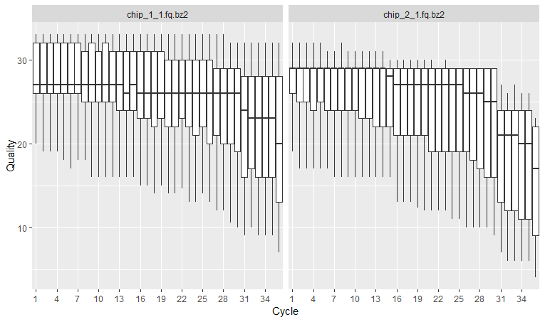
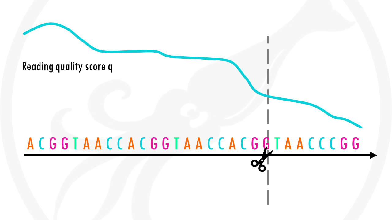
In the y axis we have the quality score, which is an estimate of the probability of that base being called wrongly q = -10 x log₁₀(p)”. So obviously we want this q-score to be as high as possible. You will often see that towards the end of the reads the quality usually decreases. It helps us decide in case we need to trim the end of the reads later on, because we cannot really trust the sequenced bases towards the start or the end of the reads. In general, a good sample will have median quality scores per base above 28. If scores are below 20 towards the ends, you can think about trimming the reads.

Per-base sequence content shows nucleotide proportions for each position or cycle. In a random sequencing library there should be no nucleotide bias and the lines should be almost parallel with each other.

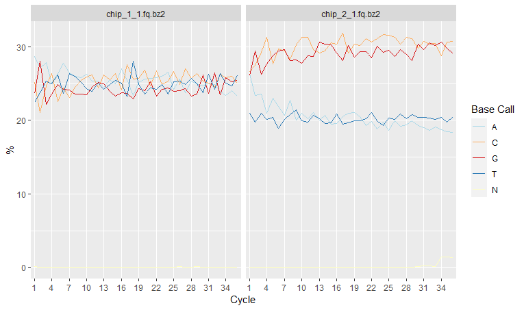
However sometimes we might detect a biased sequence composition. This could be due to several reasons:

• Some genomes are very GC biased
• Some NGS applications also introduce a strong GC bias, for example, Bis-seq.
• Some types of sequencing libraries can produce a biased sequence composition. For example, in RNA-Seq, it is common to have bias at the beginning of the reads. This happens because of random primers annealing to the start of reads during RNA-Seq library preparation. These primers are not truly random, which leads to a variation at the beginning of the reads. Although RNA-seq experiments will usually have these biases, this will not affect the ability of measuring gene expression.

Finally, the read frequency plot shows the degree of duplication for every read in the library. A high level of duplication, non-unique reads, is likely to indicate an enrichment bias. Basically, that we have a high proportion of the same sequence. This could be due to PCR artifacts that can cause technical duplicates.

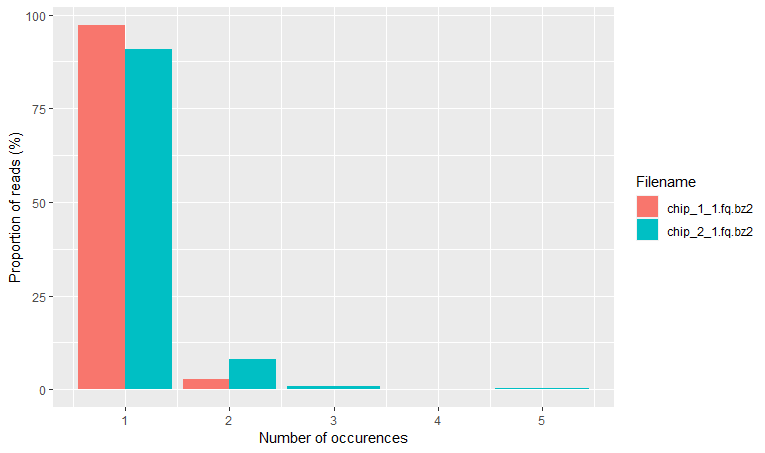
What do we mean by this?

As you know, PCR amplifies or creates many copies of a sequence fragment. In RNAseq experiments, the non-unique read proportion can be more than 20%. But these duplications can also be from genes simply being expressed at high levels. This means that there will be many copies of transcripts and many copies of the same fragment. Since we cannot be sure these duplicated reads are due to PCR bias or an effect of high transcription, we should not remove duplicated reads in RNA-seq analysis. However, in ChIP-seq experiments duplicated reads are more likely to be due to PCR bias.

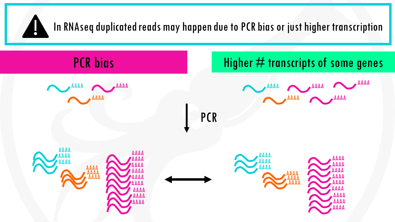
There are other quality metrics and QC tools, and again, this is only a guide for standard whole genome sequencing samples, and will be different if you are analyzing RNA-seq, bisulfite, amplicon, transposase, ATAC-seq or many other data.

I would also like to mention Fastqc, which is the most popular tool for sequencing quality control. But that is a story for another video. You can read more about FastQC and download it for free here.

Rqc package also offers the option of creating a QC report with more qc checks. I use the openFileinOS() function to open the .html file, but you can also just go to the folder and click on it to open it.

Here you will see more QC plots that might help you detect issues in your reads.

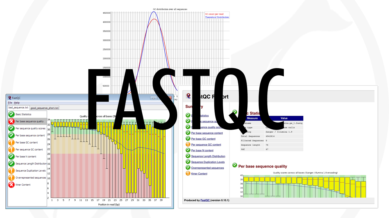
Great! You made it past the quality control checks. Now that you have a better idea of the quality of your reads, you are ready to do something about those low-quality bases – it’s time to take the scissors out and do some read trimming!

Step 2: Filtering and trimming reads

Based on the results of the quality check, you may want to trim or filter the reads.

The quality check might have shown the number of reads that have low quality scores. These reads will probably not align very well because of the potential mistakes in base calling, or they may align to wrong places in the genome. Therefore, you may want to remove these reads from your fastq file.

Another potential scenario is that parts of your reads need to be trimmed in order to align the reads. In some cases, adapters will be present in either side of the read; in other cases technical errors will lead to decreasing base quality towards the ends of the reads. Both in these cases, the portion of the read should be trimmed so the read can better align the genome.

The function we are going to use today is preprocessReads() from the QuasR package. You can check all the possibilities to preprocess reads by calling

For example, we can

• match adapter sequences and remove them.
• remove low-complexity reads (reads containing repetitive sequences).
• trim the start or ends of the reads by a pre-defined length.
• Filter reads with a certain number of unidentified bases (they are represented by the ‘N’ character.
• And more!

In our case, we will just remove reads shorter than 10 base-pairs and trim 3 bases on the 3’ end since they had quite bad quality scores if you remember. We can also remove reads that have more than 1 N.

As you can see we get a nice summary which tells us how many sequences were removed and how many are left in the end.

Great! The preprocessReads() function already offers you a lot of possibilities. But you might need something more. For example, the ShortRead package has low-level functions, which can filter reads in ways that are not possible using the preprocessReads() function.

For example, you might want to filter the reads where every quality score is below 20. In sequencing, base quality in DNA is usually measured by the Phred score. the more consistent the sequenced base is, the higher the Phred score. A Phred Score of 20 indicates the likelihood of finding 1 incorrect base call among 100 bases. In other words, the precision of the base call is 99%. So basically, we want to keep reads with a score equal or bigger than 20.

Ok, so this little bit of code is a bit more advanced but we´ll go through it step by step.

As fastq files can be quite large, it may not be feasible to read a 30-Gigabyte file into memory. A more memory-efficient way would be to read the file piece by piece. We can do our filtering operations for each piece, write the filtered part out, and read a new piece. Fortunately, this is possible using the ShortRead::FastqStreamer() function. This function enables “streaming” the fastq file in pieces, which are blocks of the fastq file with a pre-defined number of reads. We can access the successive blocks with the yield() function. Each time we call the yield() function after opening the fastq file with FastqStreamer(), a new part of the file will be read to the memory.

So this is the basic structure. Whatever we put in here will be done repeatedly for every block of the file.

But wait a minute. We have 2 files. Since you might have multiple files, I will just put all of this inside a for loop which will go though all the fasqFiles.

Instead of the name of a single file, we will loop through the fastqFiles object, which if you remember contained the names of our two files. So the first time it goes through the loop, i will equal 1, which means fastqFile will take the first value of the fastqFiles vector. Then, the fastqStreamer part combined with the yield function will allow us to take little pieces of that file, inside the while() we will have our filtering operations, and once it finishes with that file it will go back to our for loop, I will take value 2 (which in this case is the last value it will take since we only have 2 chip files), and so it will repeat everything.

And now for the actual filtering part.

We want to remove reads where all quality scores are < 20.

We first get the quality scores per base as a matrix. Then we can get the number of bases per read that have Q score < 20. Now we can check how many reads have all Phred scores bigger or equal to 20 and filter them out. Since this is inside this for loop, it will not print it out, so we can force it to print it with the print() function. We can also add the cool print() part which basically just prints out a message telling us what it’s going to print. You can check how it works and customise it to your needs, or even add more printing functions!

Now we need to write a new filtered fastq file which only contains reads where all quality scores are bigger or equal to 20. In the arguments of the function, we need to define the actual file you would like to write out, which is our filtered fastqfile. Then we have the name for the file. Since we’re inside a for loop we cannot just write ‘fastqfile_filtered’ (or any other fixed name), because then every time it runs through the for loop it will overwrite the new file with the old. So what we’ll do is take the fastqfile name and add ‘Qfiltered’ at the end. If you play around with it you will realise we need to first remove the file extension name, and add it again at the end, otherwise our file won’t be written in fastq format cause the filename will just have Qfiltered at the end instead of the extension name. It is also important to set mode = ‘a’ so that everything inside the while() function (so all the little pieces of our fastqfile) are written out to the same file.

Nice! Ok that was a bit more complicated but this structure would be a basic scaffold let’s say that would allow you to set up a nice pipeline if you have to go though many fastq files. So if you have additional filtering steps you would just add them here, before the fastq function, and that would work nicely.

Step 3: Mapping or aligning reads onto the genome

After the quality check and potential pre-processing, the reads are ready to be mapped or aligned to the reference genome. This process simply finds the most probable origin of each read in the genome. Since there might be errors in sequencing and mutations in the genomes, we may not find exact matches of reads in the genomes. That is why the previous steps of qc and filtering out low quality reads is essential. But still, alignment algorithms have to be able to tolerate potential mismatches between reads and the reference genome.

To be more time and computationally efficient, these algorithms essentially create genome indices to be able to store and efficiently search the genome for matching reads. We will not go into the details of the algorithms, but we will use a Bowtie aligner from the Rbowtie package, which is quite fast and memory efficient. You can read more about the Bowtie aligner here.

We will use the qAlign() function which requires two mandatory arguments:

• a genome file in either fasta format or as a BSgenome package and
• a sample file which is a text file and contains file paths to fastq files and sample names.

Remember the h19sub.fa file we copied at the beginning (step 0)? That is our genome file. You may want to use another reference genome for your alignment, so make sure to choose the right version (and species!) to fit your analysis.

What about the sample file? If you open up the sample file, you will see it looks something like this:

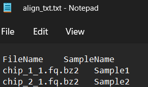
If you would like to adapt the sample file to your own sequencing files you can do it by manually editing this align_txt.txt file. But it is quite time consuming and error prone, so let’s just write a little bit of code to help us create this file for us.

First, we create a vector called ‘filenames’ where we store the names of the files we want to include. In this case, I used the original chip fastq files (not processed) and the processed ones, just to compare the final results. Of course when you build up your pipeline you might want to just use the processed ones.

As you can see in the screenshot above, we need two columns. One with the name of the files (FileNames), and the other with the name of the samples (SampleName). We can bind two vectors to create a dataframe using cbind(), then rename the columns.

And finally we write out the table to a Tab-delimited text file. The parameters you see below are essential if you want the align function to work, we want to keep the column names, but not the row names, we don’t want the elements (so our different character strings) to have quotation marks, and we need to set the separator to ‘\t’.

So now if you go to your folder you should see the table you exported.

Nice! So now we can just use the qAlign() function to align our filtered reads to the genome. You can read more about other arguments it takes which can be optimized for different alignment problems by calling ?qAlign(). For example, if you are working with bisulfite sequencing (so DNA methylation) data you will need a few extra steps to deal with the C->T conversion.

Our results are stored in this project object. You can also check that for each input sequence file, there will be one .bam file with alignments against the reference genome. BAM files contain alignment data in addition to everything contained in the fastq file.

In this tutorial we didn’t use it, but you can add an auxiliary file which contains other sequences which can be used as additional targets to align reads that do not map to the reference genome. So you might get extra bam files if they map to this auxiliary sequences.

The .bam file names consist of the base name of the sequence file with an added random string. The random suffix makes sure that newly generated alignment files do not overwrite existing ones, for example of the same reads aligned against an alternative reference genome.

Each alignment file is accompanied by two additional files with suffixes .bai and .txt. The .bai file is the bam index used for fast access by genomic coordinate. The .txt file contains all the parameters used to generate the corresponding bam file so you shouldn’t delete it, otherwise quasR won’t be able to use the bam file.

QuasR can produce a quality control report in the form of a series of diagnostic plots with details on sequences and alignments with the function qQCReport() which will export a pdf. The alignmentStats gets the number of (un-)mapped reads for each sequence file in a qProject object,

Finally, for visualization in a genome browser, alignment coverage along the genome can be exported to a (compressed) .wig file using the qExportWig() function.

And that is all for today!

I really hope this tutorial was helpful. Have a squitastic day and see you in the next one!