A step-by-step R tutorial on performing Gene Set Enrichment Analysis with R package fgsea
In this tutorial you will learn how to conduct Gene Set Enrichment Analysis (GSEA) using R-package fgsea. This package implements an algorithm for fast gene set enrichment analysis.
Following this easy, step-by-step tutorial, you will find out how to:
-
- Install and start fgsea()
- Prepare your dataset to perform GSEA
- Set the analysis parameters and run the analysis.
- View the GSEA results and get some nice plots!
If you are more of a video-based learner, you can check out my Youtube video on how to perform GSEA with fgsea() in R. Otherwise, just keep reading! And remember you can just copy the code by clicking on the top right corner of the code snippets in this post or Biostatsquid’s Github page.
Let’s dive in!
Check out my Youtube video to follow this fgsea R tutorial with me!
Before you start…
In this tutorial we will learn how to perform Gene Set Enrichment Analysis on differential gene expression results. We will use the R package fgsea() for fast preranked gene set enrichment analysis (GSEA).
If you are not that familiar with GSEA, you might want to check my other post on GSEA – simply explained! I go over the basic concepts behind GSEA algorithms and how to interpret the results.
If you are a beginner in R, don’t be overwhelmed! This tutorial will go step-by-step and I will explain (almost!) every line of code so you know what is happening at each point of the workflow.
For this tutorial you will need R, or Rstudio, and you will need to install fgsea.
Psst!
This is an updated improved tutorial that may not correspond exactly to what I initially ran when I posted the Youtube video. If you want to stick to the older version, you can check it out here.
Install fgsea()
You can read more about fgsea() package here. To install fgsea, use the following command:
BiocManager::install("fgsea")Once installed, we can load the package:
library("fgsea")Set up your environment
It’s good practice to clear up your environment before you load in any data. This is the general structure I like to keep in all my scripts:
# ----------------------
# GSEA tutorial
# ----------------------

# Setting up environment ===================================================
# Clean environment
rm(list = ls(all.names = TRUE)) # will clear all objects including hidden objects
gc() # free up memory and report the memory usage
options(max.print = .Machine$integer.max, scipen = 999, stringsAsFactors = F, dplyr.summarise.inform = F) # avoid truncated output in R console and scientific notation

# Set seed
set.seed(123456)

# Loading relevant libraries
library(tidyverse) # includes ggplot2, for data visualisation. dplyr, for data manipulation.
library(RColorBrewer) # for a colourful plot
library(fgsea)
library(msigdbr)

# Set relevant paths
project_path <- "C:/Users/laura/Documents/Biostatsquid/Projects"
in_path <- file.path(project_path, 'data/scRNAseq') # DGE results path
out_path <- file.path(project_path, "PEA/Results") # GSEA output path
bg_path <- file.path(project_path, "Background_genes") # path to your downloaded background genes
dir.create(out_path, showWarnings = F, recursive = T)
What do I need to run fgsea?
Essentially, there are two things you need to perform preranked gene set enrichment analysis with fgsea.
The fgsea package takes in two main arguments.
The first one is pathways: a list of gene sets or pathways to check
The second one is stats: a named vector of our genes of interest we want to perform GSEA on. The gene names must be the same as the ones in pathways! So make sure you are using the same nomenclature (i.e., gene IDs or Ensemble IDs).
That’s it!
There are additional parameters you may be interested in such as:
- minSize: minimal size of a gene set to test (all pathways below the threshold are excluded)
- maxSize: the same, but a maximum threshold.
- scoreType: the default is ‘std’, where the enrichment score is computed normally, but you can also use one-tailed tests if you are only interested in positive (‘pos’) enrichment – so only pathways that are overrepresented – or negative (‘neg’) enrichment – to only get pathways that are underrepresented in your list of genes.
1. Prepare your gene sets / pathways
As we already saw in the Pathway Enrichment Analysis with clusterProfiler() tutorial, we need to prepare a list of pathways
1. Get your gene set .gmt file. In my old version (and in the video), I used to download the .gmt files with the pathways manually from the msigdb database. Now, it’s so much easier! You can use the R package msigdbr to download whichever pathways you’re interested in. If you are unsure which one is right for you, check out this other post where I explain the different pathways and gene sets available in msigdb.
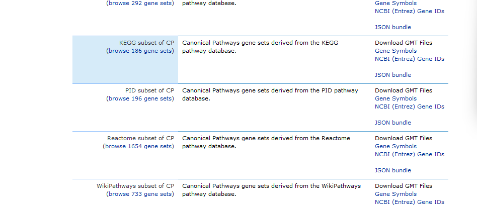
Make sure to download the gene sets that are appropriate for your analysis, and edit the species if needed!
## 2. Prepare background genes -----------------------------------------------
# msigdbr R package provides Molecular Signatures Database (MSigDB) gene sets
# Read more here: https://igordot.github.io/msigdbr/articles/msigdbr-intro.html
# msigdbr_collections()
gene_sets_df <- msigdbr(species = 'Homo sapiens', category = 'H')
#gene_sets_df <- msigdbr(species = 'Homo sapiens', category = 'C5', subcollection = 'GO:BP')
head(gene_sets_df)
2. Get the background genes ready for fgsea. As I explain in my previous post, we need to use a set of background genes that contain only the genes present in our dataframe, to avoid bias. The good news is, fgsea takes care of this! The fgsea function automatically intersects each gene set with the genes in your ranked list. If a gene in a pathway is not present in your ranked list, fgsea ignores it for that analysis. That’s why it’s important to include all the genes that were present in your dataset in your background (not only those that were upregulated, for example).
The only thing we need to do is convert the table gene_sets_df we downloaded with msigdb, to the correct format, a list:
# Convert to named list format required by fgsea
gene_sets <- gene_sets_df %>%
  split(x = .$gene_symbol, f = .$gs_name)

cat(paste("Loaded", length(gene_sets), "gene sets\n"))Squidtip
The fgsea package also provides a function that returns a list of Reactome pathways for a given vector of Entrez gene IDs.
Just call reactomePathways(genes).
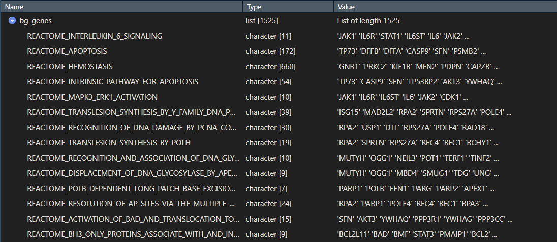
Your gene_sets object should be a list with your pathway or gene set names, and the genes that make up each pathway.
2. Prepare your ranked list of genes
We would like to perform GSEA on our differentially expressed genes. Unlike pathway enrichment analysis, GSEA provides the advantage of not needing to subset our gene list. We can provide all the genes that resulted from our differential expression analysis. Even genes that were not significantly differentially expressed.
We just need to rank our genes first.
The way it works is, you need to give fgsea a named vector with the rankings and the genes symbols as names.
If you are not very clear on this, you might want to check out my post on GSEA – simply explained!
Squidtip
How do you rank your genes?
There are many ways of ranking your genes, so you need to decide based on your analysis. Here, I use the sign(df$log2fc)*(-log10(df$pval))) as a ranking metric.
This way, the magnitude of the ranking will be given by the p value (since I use -log10(), the more significant a gene is differentially expressed, the larger that value will be). The sign of the ranking (positive or negative) will be given by the fold-change: upregulated genes will have positive rankings, downregulated genes will have negative rankings.
## 1. Read in data -----------------------------------------------------------
list.files(in_path)
df <- read.csv(file.path(in_path, 'severevshealthy_degresults.csv'), row.names = 1)
head(df)
# gene_symbol      pval      padj               log2fc
# 1 MIR1302-2HG 0.9998587 0.9999881 15.86284051374880022
# 2     FAM138A 0.9999881 0.9999881 -0.00000000000283586
# 3       OR4F5 0.9999881 0.9999881 -0.00000000000283586
## 3. Prepare ranked list of genes -----------------------------------------------
## FGSEA needs a named vector with the rankings and the genes as names
## We will use signed p value as ranking: sign(df$log2fc)*(-log10(df$pval)))
# Note that you can also just use the log2FC only - but it will not take into account
# genes with a large FC but non-significant
rankings <- sign(df$log2fc)*(-log10(df$pval)) # we will use the signed p values from spatial DGE as ranking
names(rankings) <- df$gene_symbol # genes as names#Easy! We’ve just created our ranked list of genes.
You can have a look at the values:
> head(rankings)
    MIR1302-2HG         FAM138A           OR4F5      AL627309.1      AL627309.3      AL627309.2
 0.000061381930 -0.000005164293 -0.000005164293 -0.154354567687 -0.000005164293 -0.000005164293
> rankings <- sort(rankings, decreasing = TRUE) # sort genes by ranking
> plot(rankings)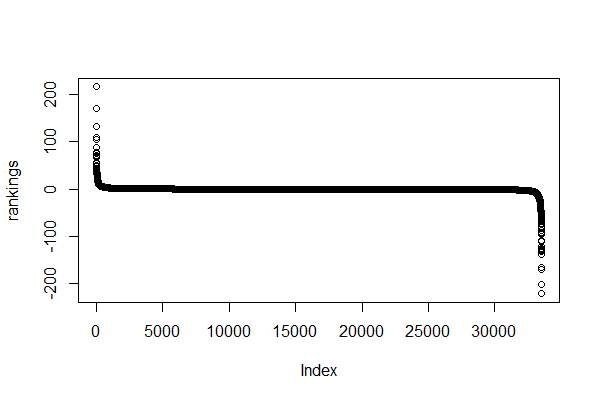
Yes, it’s an ugly plot, I know.
In the x axis, we see our genes (each dot represents a gene) – they are indexed so instead of gene symbols we just see numbers from 1 to 33538.
In the y axis, we see the ranking (sign(df$log2fc)*(-log10(df$pval)))) for each gene.
Squidtip
Another note on rankings… You can just use the log2(fold-change) as a ranking – but it will not take into account genes with a large fold change but non-significant. However, if you have already selected your significant genes, this may be a good option for you.
Most genes have a ranking value between -100 and 100.
A few ones seem to have higher rankings. Let’s have a closer look…
> max(rankings)
[1] Inf
> min(rankings)
[1] -Inf
It seems like some genes have a ranking of infinity. This is due to the fact that some p-values were really small, so computing -log10(p-value) returned infinity.
fgsea() does not accept non-finite numbers as rankings, so we need to fix that.
In this case, we will just convert them to really large (or small) values:
# Some genes have such low p values that the signed pval is +- inf, we need to change it to the maximum * constant to avoid problems with fgsea
max_ranking <- max(rankings[is.finite(rankings)])
min_ranking <- min(rankings[is.finite(rankings)])
rankings <- replace(rankings, rankings > max_ranking, max_ranking * 10)
rankings <- replace(rankings, rankings < min_ranking, min_ranking * 10)
rankings <- sort(rankings, decreasing = TRUE) # sort genes by ranking
By replacing the infinite values by ten times the maximum or minimum ranking, we avoid errors when running fgsea().
Now, if we plot the rankings:
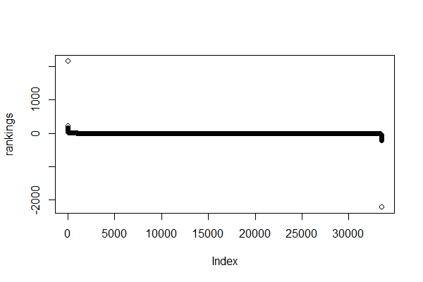
> max(rankings)
[1] 2152.518
> min(rankings)
[1] -2206.971
You can also check the rankings of a specific set of genes and a nicer plot with ggplot.
Let’s have a look at the first 50 genes (if you don’t have many genes you can try with all but since I have 33538 I don’t want it to crash – again).
ggplot(data.frame(gene_symbol = names(rankings)[1:50], ranks = rankings[1:50]), aes(gene_symbol, ranks)) +
	geom_point() +
	theme_classic() +
	theme(axis.text.x = element_text(angle = 90, vjust = 0.5, hjust=1))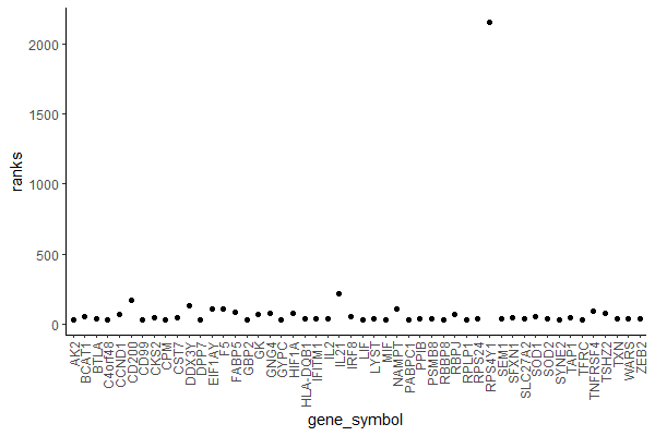
3. Run GSEA
## 4. Run GSEA ---------------------------------------------------------------
# Easy peasy! Run fgsea with the pathways
GSEAres <- fgsea(pathways = gene_sets, # List of gene sets to check
                 stats = rankings,
                 scoreType = 'std', # in this case we have both pos and neg rankings. if only pos or neg, set to 'pos', 'neg'
                 minSize = 10,
                 maxSize = 500,
                 nproc = 1) # for parallelisation
You might get a warning saying:
Warning message:
In preparePathwaysAndStats(pathways, stats, minSize, maxSize, gseaParam,  :
  There are ties in the preranked stats (48.8% of the list).
The order of those tied genes will be arbitrary, which may produce unexpected results.
As it states there, there are many genes with ‘tied’ scores or rankings. Genes with the same score will just be ordered at random by the algorithm, and might slightly affect your results when computing the Enrichment Score. This just means that if genes #15 # 16 and #17 have a ranking of ’10’, they will be ordered at random (#17 #15 #16).
It shouldn’t have a very big effect on your results. In my case, it mostly affects genes with a ranking near 0 (they were not significant genes).
Squidtip
About the scoreType… If you have only positive rankings, you can change this to ‘pos’. For example, if you are using the absolute value of logFC. It is not very common, but you can read more about use cases here.
> head(GSEAres)
                                                                                pathway      pval      padj    log2err
1:                                           REACTOME_ABACAVIR_TRANSPORT_AND_METABOLISM 0.3633218 0.9085975 0.08862611
2:                                      REACTOME_ABC_FAMILY_PROTEINS_MEDIATED_TRANSPORT 0.4397394 0.9085975 0.11573445
3:                                       REACTOME_ABC_TRANSPORTERS_IN_LIPID_HOMEOSTASIS 0.9746835 0.9856000 0.05773085
4:                                                   REACTOME_ABC_TRANSPORTER_DISORDERS 0.3471338 0.9085975 0.13077714
5:            REACTOME_ABERRANT_REGULATION_OF_MITOTIC_EXIT_IN_CANCER_DUE_TO_RB1_DEFECTS 0.9820051 0.9882600 0.05809836
6: REACTOME_ABERRANT_REGULATION_OF_MITOTIC_G1_S_TRANSITION_IN_CANCER_DUE_TO_RB1_DEFECTS 0.5102564 0.9085975 0.09167952
           ES        NES size                             leadingEdge
1: -0.7980657 -1.1339616   10                                   ABCB1
2:  0.4951437  0.9782602  103  PSMB8,SEM1,PSMB9,PSMB3,PSMA6,PSME1,...
3:  0.3593687  0.5781693   18     PEX3,ABCG1,APOA1,ABCG8,ABCA3,ABCA10
4:  0.5572234  1.0724269   78  PSMB8,SEM1,PSMB9,PSMB3,PSMA6,PSME1,...
5:  0.3580019  0.5778174   20 ANAPC5,ANAPC2,CDC26,CDC27,UBE2C,RB1,...
6:  0.6152041  0.9756658   17                       CCND1,CCND3,CCNE1
4. Visualise your GSEA results
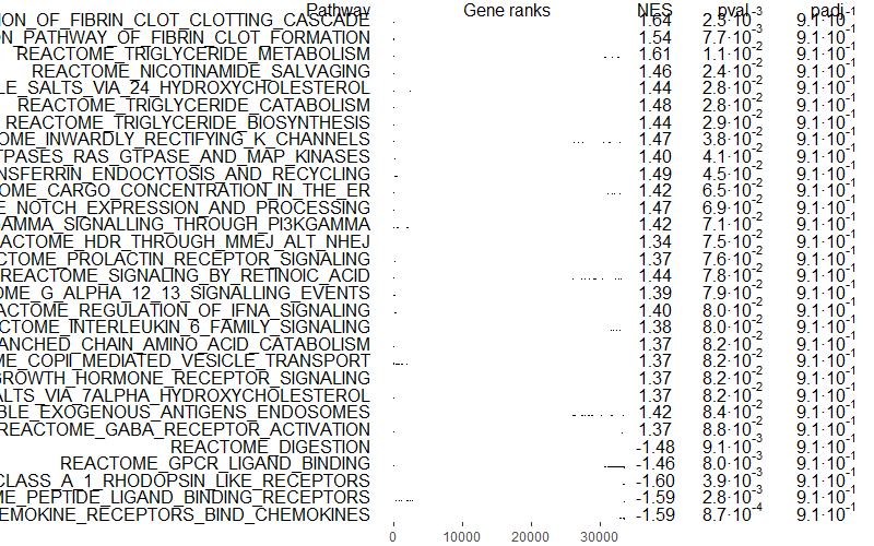
Let’s have a look at our top 6 enriched pathways, ordered by p-value or p-adjusted value.
## 6. Check results ------------------------------------------------------
# Top 6 enriched pathways (ordered by p-val)
head(GSEAres[order(pval), ])
How many significant pathways did we get?
> sum(GSEAres[, padj < 0.01])
[1] 0
> sum(GSEAres[, pval < 0.01])
[1] 8
Clearly, our results are not great. There are only 8 significant pathways (p-value < 0.05), but when correcting for multiple testing, we have no significant pathways (p-adjusted values < 0.05).
Oh, well. For the sake of this tutorial, let’s keep going! Hopefully your results will be prettier than mine…
Let’s plot our top pathways. I ordered them by p-value because my pathway enrichment analysis did not yield very interesting results… but you can change it to p-adjusted values if you would like to be more restrictive and correct for multiple testing…
number_of_top_pathways_down <- 10 # Choose how many downregulated pathways you would like to display
number_of_top_pathways_up <- 10 # Choose how many upregulated pathways you would like to display

topPathwaysUp <- GSEAres[ES > 0][head(order(pval), n = number_of_top_pathways_up), pathway]
topPathwaysDown <- GSEAres[ES < 0][head(order(pval), n = number_of_top_pathways_down), pathway]
topPathways <- c(topPathwaysUp, rev(topPathwaysDown))
#pdf(file = paste0(filename, '_gsea_top30pathways.pdf'), width = 20, height = 15)
plotGseaTable(gene_sets[topPathways], stats = rankings, fgseaRes = GSEAres, gseaParam = 0.5)
#dev.off()
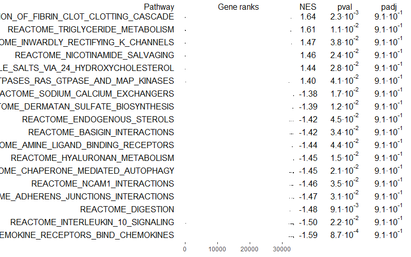
You can also select only independent pathways, removing redundancies or similar pathways with the function collapsePathways():
# Select only independent pathways, removing redundancies/similar pathways
collapsedPathways <- collapsePathways(GSEAres[order(pval)][pval < 0.05], gene_sets, rankings)
mainPathways <- GSEAres[pathway %in% collapsedPathways$mainPathways][order(-NES), pathway]
#pdf(file = paste0('GSEA/Selected_pathways/', paste0(filename, background_genes, '_gsea_mainpathways.pdf')), width = 20, height = 15)
plotGseaTable(gene_sets[mainPathways], rankings, GSEAres, gseaParam = 0.5)
#dev.off()
Squidtip
If you’d like to export the tables, just uncomment the 2 lines above. You can also export to .png, or other formats:
png(file = paste0(filename, ‘_gsea_mainpathways.png’), width = 1500, height = 800)
plotGseaTable(gene_sets[mainPathways], rankings, GSEAres, gseaParam = 0.5)
dev.off()
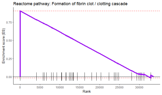
Now let’s plot the ES of the most significantly enriched pathway.
# plot the most significantly enriched pathway
plotEnrichment(gene_sets[[head(GSEAres[order(padj), ], 1)$pathway]],
               rankings) +
  labs(title = head(GSEAres[order(padj), ], 1)$pathway)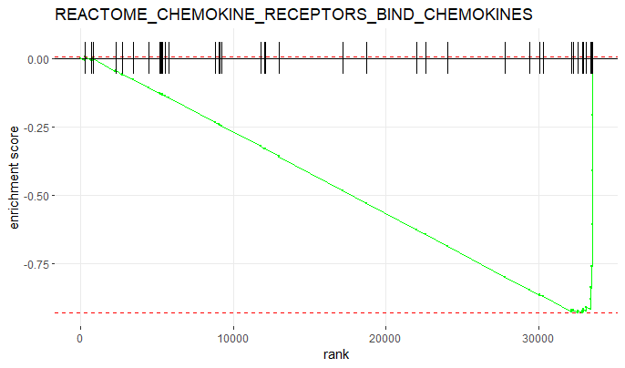
You can also edit the plot and make it prettier;)
plotEnrichment(gene_sets[['REACTOME_FORMATION_OF_FIBRIN_CLOT_CLOTTING_CASCADE']],
               rankings) +
  labs(title = 'Reactome pathway: Formation of fibrin clot / clotting cascade') +
  theme_classic() +
  scale_x_continuous('Rank', breaks = seq(0, 32000, 5000)) +
  scale_y_continuous('Enrichment score (ES)') +
  geom_line(col = 'purple', linewidth = 2)
5. Save your results
## 5. Save the results -----------------------------------------------
name_of_comparison <- 'severevshealthy'
background_genes <- 'gobp'
filename <- paste0(out_path, 'GSEA/', name_of_comparison, '_', background_genes)
#saveRDS(GSEAres, file = paste0(filename, '_gsea_results.RDS'))
#data.table::fwrite(GSEAres, file = paste0(filename, '_gsea_results.tsv'), sep = "\t", sep2 = c("", " ", ""))
sessionInfo()
Check my sessionInfo() here in case you have trouble reproducting my steps:
> sessionInfo()
R version 4.2.3 (2023-03-15 ucrt)
Platform: x86_64-w64-mingw32/x64 (64-bit)
Running under: Windows 10 x64 (build 22621)

Matrix products: default

locale:
[1] LC_COLLATE=English_Ireland.utf8  LC_CTYPE=English_Ireland.utf8
[3] LC_MONETARY=English_Ireland.utf8 LC_NUMERIC=C
[5] LC_TIME=English_Ireland.utf8

attached base packages:
[1] stats     graphics  grDevices utils     datasets  methods   base

other attached packages:
 [1] fgsea_1.24.0       RColorBrewer_1.1-3 lubridate_1.9.2    forcats_1.0.0
 [5] stringr_1.5.0.9000 dplyr_1.1.2        purrr_1.0.1        readr_2.1.4
 [9] tidyr_1.3.0        tibble_3.2.1       ggplot2_3.4.2      tidyverse_2.0.0

loaded via a namespace (and not attached):
 [1] Rcpp_1.0.11         pillar_1.9.0        compiler_4.2.3      tools_4.2.3
 [5] lattice_0.20-45     lifecycle_1.0.3     gtable_0.3.3        timechange_0.2.0
 [9] pkgconfig_2.0.3     rlang_1.1.1         Matrix_1.5-3        fastmatch_1.1-3
[13] cli_3.6.0           rstudioapi_0.14     parallel_4.2.3      withr_2.5.0
[17] generics_0.1.3      vctrs_0.6.3         hms_1.1.3           cowplot_1.1.1
[21] grid_4.2.3          tidyselect_1.2.0    data.table_1.14.8   glue_1.6.2
[25] R6_2.5.1            fansi_1.0.4         BiocParallel_1.32.6 farver_2.1.1
[29] tzdb_0.4.0          magrittr_2.0.3      codetools_0.2-19    scales_1.2.1
[33] colorspace_2.1-0    labeling_0.4.2      utf8_1.2.3          stringi_1.7.12
[37] munsell_0.5.0
And that is the end of this tutorial!
In this post, I explained how to perform gene set enrichment analysis using fgsea. Hope you found it useful!
Before you go, you might want to check:
Squidtastic!
You made it till the end! Hope you found this post useful.
If you have any questions, or if there are any more topics you would like to see here, leave me a comment down below.
Otherwise, have a very nice day and… see you in the next one!
Squids don't care much for coffee,
but Laura loves a hot cup in the morning!

If you like my content, you might consider buying me a coffee.
You can also leave a comment or a 'like' in my posts or Youtube channel, knowing that they're helpful really motivates me to keep going:)
Cheers and have a 'squidtastic' day!


Great tutorial! Much appreciated!
in Python and/or R, how can we visualize timeseries (Day 1 to 5) of the difference of gene expression by outcome (Survivor / Non-Survivor)?
Hi Claude, thanks for your feedback! That’s a really good question. I don’t have experience with timeseries data, but here are a few resources that may inspire you:
https://bmcbioinformatics.biomedcentral.com/articles/10.1186/s12859-017-1647-3 -> has some visualisation plots
https://academic.oup.com/bib/article/20/1/288/4364840 -> has some bioinformatic tools
https://software.broadinstitute.org/cancer/software/gsea/wiki/index.php/FAQ#Can_I_use_GSEA_to_analyze_time_series_data.3F –> just found this, might answer your question?
Hope it helps!:)
PS. If you are looking at a particular gene (or just a few of them), it might be as simple as plotting a lineplot grouped by outcome, with log2FC of the specific DEG in the y axis, time in the x axis, and you could also have the colour as a function of the p-values (or maybe if it is significantly differentially expressed at all timepoints, you don’t need this) – you could do this with ggplot quite easily.
great tutorial!! but I have a problem with the last line of the final graphic:
geom_line(col = ‘purple’, linewidth = 2), error in `compute_geom_1()`:
! `geom_line()` requires the following missing aesthetics: x and y
Hi! Thanks so much for your comment. Hmm, that’s strange – did you specify x and y in the main function’s aesthetics? I mean when you call ggplot(… aes(x = , y = )).
Otherwise, you can also specify them again in the geom_line() function. This is what I mean: https://community.rstudio.com/t/error-geom-point-requires-the-following-missing-aesthetics-x-y/26224
Hope it helps!
Great tutorial ! Do you know of a citation for using a combination of pvalue and fold change as a ranking criteria ?
Thank you for your comment! Yes, I’m pretty sure there’s more publications but here’s one where they propose the method I use in the tutorial: https://www.ncbi.nlm.nih.gov/pmc/articles/PMC3957066/
Cheers!
Hi, thank you for your tutorial! I got the following error while running the prepare_gmt function for bg_genes:
Error in colSums(mat[hidden1, ]) :
‘x’ must be an array of at least two dimensions
In addition: Warning message:
In readLines(gmt.file) :
incomplete final line found on ‘PEA/Background_genes//HALLMARK_NOTCH_SIGNALING.v2023.2.Hs.gmt’
Am I doing something wrong here?
Hi! Thanks for your comment – are you use that’s the path were the file is located?
Try list.files(‘PEA/Background_genes/’) – does R return that file? If no, then you need to provide the folder/path were the file is. If yes, then maybe try checking if the file looks ok size-wise and if not try downloading the file again? Code seems to work for me!
Hi thanks for the tutorial! I’m not very experienced with R but I’m trying to perform this fgsea. I’m getting stuck on step 1.2 when it comes to reading the gmt file and then intersecting. Are the objects “gmt” and “genes_in_data” defined elsewhere?
Hey Julia! Thanks for your question. So the first step is to download a gmt file, which I explain in 1.1. Then you have to save the file(s) you download in whichever folder you want. In my case, I saved it in PEA/Background_Genes.
You need to make sure R is able to read in this file, so make sure the folder is defined properly (you might need to give it the full path, e.g., ‘C:/Users/…). You can check if R has access to the folder with
foldername <- 'C:/Path/to/my/folder' list.files(foldername) This should return all the files in your folder. About genes_in_data - so sorry! That was on my end. I copied the lines from the function I post a few lines below (prepare_gmt) and genes_in_data is the argument for that function. If you see at the very end of that snippet when I call the function, I pass my_genes as the argument genes_in_data. It's a bit confusing if you are not used to functions, but in summary, use my_genes. I will correct it in the snippet so it's not confusing - thanks for your comment!!
Hi,
I have facing issue in collapsedPathways function as follow :
> collapsedPathways <- collapsePathways(GSEAres[order(padj)][padj < 0.01], bg_genes, rankings)
Error in preparePathwaysAndStats(pathways, stats, minSize, maxSize, gseaParam, :
Not all stats values are finite numbers
could you please help me to sort this out ?
Hi – would need more info to reproduce the error but maybe this will help: https://www.biostars.org/p/9557480/
Hi.thank you for your great tutorial.
id did not underestand one thing.
how can i annotate most significant genes of every pathways in R(leading edge subset of genes)
im so sorry.it was stored in the results.is did not see it at first 🙁
Hello, i am having trouble to understand why don’t we have a .cls phenotype file in order to choose what we want to compare ? In my case i have 4 phenotypes and i want to compare two. How does this work?
Here are my file:
Gene expression data .gct/.txt
geneset .gmx/.gmt
Phenotype data .cls
pre-ranked genelist .rnk
Hi, thanks for your comment! Not sure I understand your question, but if there is only two groups you want to compare, you might want to filter them first.
Hello. Thanks for the great tutoring. I am running the code, but I am getting the bg_genes back as a list() – so it does not have any components to it. When I then run the fgsea, I am getting 0 observations. Do you have any comments on this? Thanks so much.
Hi – thanks for your comment! You need to download the background gene set and read it into R – I explain it in the first steps of the tutorial. It seems like you are not reading this into R properly – maybe just a quick fix with your paths? To make sure that the data is there and R can “see” it – you can use list.files(/your/path/to/wherever/you/saved/the/background/files).
Hi, Great tutorial, thank you so much! I was wondering whether you have any comments on how to plot the results in a bar chart format? Is this possible?
Thank you!
Hi thanks for your comment, you’re very welcome:) For sure it’s possible – but what would you like to plot? Barplots are usually useful to show a numerical distribution of categorical data – for example, in the x axis you could have your top significant pathways, and in the y axis the gene count or ratio as bar heigh/colour? You have an example here, with clusterProfiler: https://biostatsquid.com/pathway-enrichment-analysis-plots/
But you would have to build it with ggplot (really easily!) using geom_bar()
Let me know if you think it would be useful to have a tutorial on this:)
Hii, im really stuck while doing the analysis of the plots
The plot that was obtained consist of all the erichment scores plotted with the gene rank for a single significantly enriched pathway ? But as the fgsea result consist of only a single enrichment score for a single pathway, the how come the plot has different peaks? Sorry im a bit confused.
Hi, I’m not quite sure what you mean. If you are referring to the last plot, the x axis shows the genes, in order (ranked by sign(df$log2fc)*(-log10(df$pval)) ), the y axis shows the ES for each of the gene. This is, as you correctly pointed out, for a single pathway. You would be able to get a plot like this one for each of the pathways. Hopefully this helped! You might want to watch my youtube video on GSEA or read the blogpost https://biostatsquid.com/gene-set-enrichment-analysis/, it might be clearer then:)
Hi, I thoroughly enjoyed the video; it proved to be incredibly insightful. I am grateful for the valuable information it provided. Furthermore, I have a question to pose.
Below is the content I received this error message. How can I resolve it?
> plotEnrichment(bg_genes[[‘REACTOME_TRANSLATION’]],
+ rankings) +
+ labs(title = ‘Reactome pathway: REACTOME_TRANSLATION’) +
+ theme_classic() +
+ scale_x_continuous(‘Rank’, breaks = seq(0, 32000, 5000)) +
+ scale_y_continuous(‘Enrichment score (ES)’) +
+ geom_line(col = ‘purple’, linewidth = 2)
Error in `geom_line()`:
! Problem while setting up geom.
ℹ Error occurred in the 6th layer.
Caused by error in `compute_geom_1()`:
! `geom_line()` requires the following missing aesthetics: x and y.
Run `rlang::last_trace()` to see where the error occurred.
Hi! Thanks for your comment! Hmm, not sure why it’s not working for you, looks like you need to specify the x and y variables inside aes() – could you check that you are using the same versions of the packages I use? Otherwise just delete the geom_line() line and it should work without colouring it purple:)
Hi,
great tutorial. I want to do fgsea, but from the resulting gene list is it possible to separate the upregulated and downregulated genes/pathways? I’m confused how to do this, would it be by separating using the normalised enrichment score, so if its less than 0 this would indicate genes in that pathway have been down regulated and if larger, these are pathways with genes that are upregulated? I intend to make a 3 way venn diagram comparing the number of up and downregulated pathways across 3 different groups, but wasn’t sure the most efficient way to do so. Unless pathway enrichment is easier?
Thanks,
Hi, thanks for your comment! Not sure what you mean – could you explain further? One thing is upregulated/downregulated pathways, another is genes.
But, if I get your question right, I would do dge analysis on the 3 groups separately (vs a control group?) – then do fgsea on the 3 gene lists separately.
Hello, thank you for your tutorial. I am having trouble to find out gene sets/pathway for rat. The page you suggested have only human and mouse. Do you know else where I can find that file (ie. get) for other species (especially Rat in my case)?
Many thanks
Hi! Thanks so much for your comment. I’ve never worked with rat samples but here are some interesting papers/tools that may be useful:
https://www.ncbi.nlm.nih.gov/pmc/articles/PMC8982048/
https://www.genome.jp/kegg-bin/show_organism?menu_type=pathway_maps&org=rno
https://rgd.mcw.edu/GO/
https://reactome.org/content/schema/instance/browser/48895
Good luck!
HI! Thank you so much for this workflow, it has proven to be really useful.
I performed the GSEA over a microarray results comparing 3 experimental groups to obtain enriched reactome pathways for each one. Now I have selected the common identified pathways for the three experimental groups and I am looking for the best way to present this. I have seen other people do a kind of plot like plotEnrichment, but combining several pathways in the same plot. Is it possible to do that, but combine the three plots for each pathway? It would be very useful to compare the enrichment score and the distribution of genes in the ranked list for each of the experimental groups before following the analysis and going deeper to explore the “leading edges”.
Thank you very much for your time and again for providing all this information! 🙂
That’s a great idea for visualisation! You can definitely do that although you’ll need to tweak the code a little. I think the quickest way to do what you’ve explained would be to merge the PEA results from 3 experimental groups in a single dataframe, and rename the pathways with “Experimentalgroupname_pathwayname”. Then, plot the results using this annotation. Just make sure that what you are plotting makes sense, i.e., that you are not comparing apples to pears! Depends on how you set up your experiment but you might not be able to compare the ES directly across groups.
In the prepare_gmt function, the line :
mat 5)] ]
creates an error when just testing it with 1 gmt file. I get the error:
Error in h(simpleError(msg, call)) :
error in evaluating the argument ‘x’ in selecting a method for function ‘which’: ‘x’ must be an array of at least two dimensions
How do I fix this?
I’m also unclear on how I modify the function to read in all the pathways. Can you explain?
Hi it’s hard to know without seeing the actual code, but the error you are getting suggests that the function you’re using requires an input array or matrix with at least two dimensions (e.g., a data frame, matrix, or array), but it’s receiving a one-dimensional object (like a vector). Try running it with the example data in the blogpost and see how your objects differ. Good luck!
Hi thanks for the tutorial! I don’t get how you can read in the .gmt and the beginning by simply running ‘gmt_file <- "PEA/Background_genes/c2.cp.kegg.v7.5.1.symbols.gmt"'.
I tried to do it, but it creates a char vector.
Hey thanks for your comment, good catch! The script itself was correct, but I must have deleted it by mistake when copying it onto the blog snippet. Thanks for letting me know!
It’s fixed now, you can read it with gmt <- gmtPathways(gmt_file) PS. Actually, there's a much easier way to download and load pathways into R - you can use the R library msigdbr # Example: Download Hallmark pathways for human msig_hallmark <- msigdbr(species = "Homo sapiens", category = "H")
Hi, Thanks for a great tutorial!
I am afraid there is some alien script in the text. In “2. Prepare your ranked list of genes”chapter there is the following text, which doesn’t suit:
” …Offering popular women’s necklaces such as pendants, chokers and. Shop for jewelry in a variety of metals and gemstones to suit any occasion.”
Thanks! and oops, don’t know how that got there, fixed now! Thanks for letting me know:)
Hi Dr. Squid, thanks for this great tutorial. Just wanted to draw your attention to a couple bugs in the code on this page that I think are stemming from your conversion from the old MSigDB file downloading approach versus the new one here. Specifically, you have a couple references still to bg_genes, which it seems should be renamed to the gene_sets variable you use throughout the updated tutorial here. I think most of the discrepancies start in Section 4.
Separately, in Section 1.2, it looks like some of the header text from the old tutorial relating to using a function to select the desired .gmt file is still present, even though you’ve removed the corresponding code blocks since they are no longer relevant to the approach described in the updated tutorial.
On a less-important note, it may be helpful to include a comment in Section 4 Code Block 3 (the part where you create the top_pathways object) directing people to replace n = number_of_top_pathways_up and _down with their desired number for n? I may have missed it here, but I don’t think we’ve instantiated a number_of_top_pathways_up variable, and a novice may find it confusing if they run into a missing variable error when simply copy-pasting code. Or perhaps, this should be intuitive enough 🙂
Thanks again for this excellent tutorial, this was really helpful in getting up to speed on GSEA!
Thanks a million! This feedback was so helpful!! Incorporated all your suggestions. Cheers and have a great day:)