
A simple explanation of what is multiple testing and how it can negatively affect your data. We will also cover some of the most common multiple testing correction methods.
In this post I will try to give you a simple and practical explanation of multiple testing.
Multiple testing is one of the most common problems in biostatistics and computational biology. Luckily, there are many ways to correct it.
I will give you several examples of situations where we need to correct for multiple testing, and the advantages and disadvantages of each method.
If you are more of a video-based learner, you can check out my Youtube video, otherwise, just keep reading!
Let’s dive in!
What is multiple testing?
Making multiple comparisons means multiple chances for a false positive.
Look at what happened with the jelly beans.
When trying to find out if a particular colour of jelly beans caused acne, we tested 20 different colours.
Even if we use a p-value threshold lower than 0.05 (p-val < 0.05), this means there is a 5% chance of false positive – and that is exactly what happened.
One of the colours – red – was significantly linked to acne. Just by chance, it happened to be falsely positively correlated to getting acne.
If we did a ten page survey about nuclear power plant proximity, milk consumption, age, number of pets, favorite ice cream flavour, musical taste current sock color, and a few dozen other factors for good measure, and you will find that something is significantly correlated to cancer.

In one sentence,
The more tests, the more chance of observing at least one significant result, even if it is actually not significant.
In biology, we often don’t just do 20 tests, but thousands. Imagine the amount of false positives, even if we lower the p value to 0.01.
Thank goodness we have techniques to correct for multiple comparisons.

Multiple testing correction methods
The Bonferroni correction
The Bonferroni correction method says that if you make n comparisons, you should use a threshold of p < 0.05/n.

Imagine we want to test 1000 genes to see if they are correlated to being a morning person versus a night owl.
We might choose a p value threshold of 0.05. This means that the probability of saying that a gene is significant when it actually is not, is 5%. We’re taking a 5% chance of being wrong – of saying a gene is linked to being a morning person when it is actually not.

5% are pretty good odds, and it would be fine if it were 1 gene. The problem is we are not testing 1 gene, but 1000. This already means that up to 50 genes will be wrongly classified as significant.

With the Bonferroni correction, we use a p-value threshold of 0.05/1000, so 0.00005. There is 0.005% chance that we are wrong and the gene is actually not associated with being a morning person.
The problem with the Bonferroni correction, is that it is too conservative. Yes, it lowers the chances of false positives, but we are also demanding much stronger correlations before you conclude they’re statistically significant. So we get a lot of false negatives: genes that are less strongly correlated, will not be considered at all. In a nutshell, we might miss a lot of interesting genes.

Time for another example.
To make it easier to visualise, let’s not talk about genes, but going to the beach.
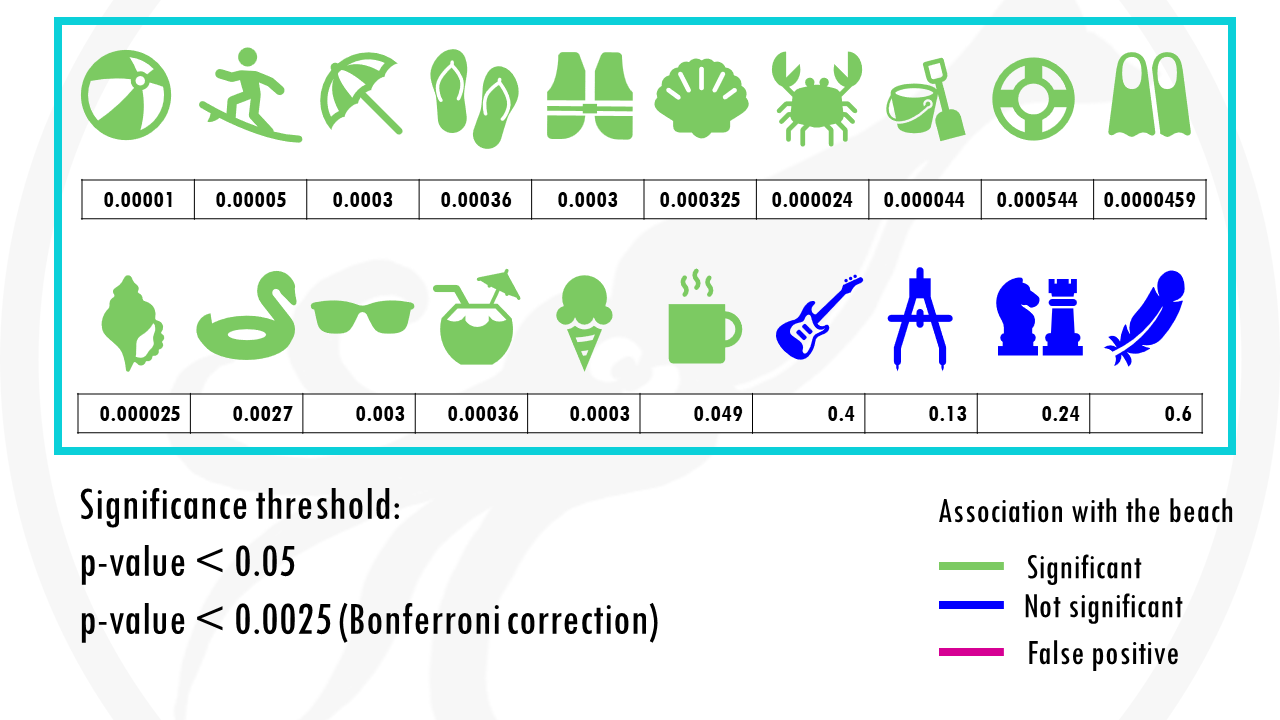
We test 20 different objects to see if they are associated with the beach.
After choosing the appropriate statistical test, we get a p-value for each object, indicating how statistically significant is there association to the beach.
If we set a p value threshold of 0.05, it means 15 objects were significantly linked with the beach, and 5 of them were not.

Some objects, like sunglasses or a towel, have really low p values, because they are strongly correlated with going to the beach. Our p-value threshold is 0.05, meaning there is still a 5% probability that we classify an object as being correlated with going to the beach, when actually it is not, just by chance.
And this is exactly what happened.
The cup of coffee was found statistically significant, when in fact, it is not correlated with going to the beach.
(If you are one of those people who always takes a cup of coffee to the beach and thinks both are totally linked, just pretend it’s not for the sake of the example).

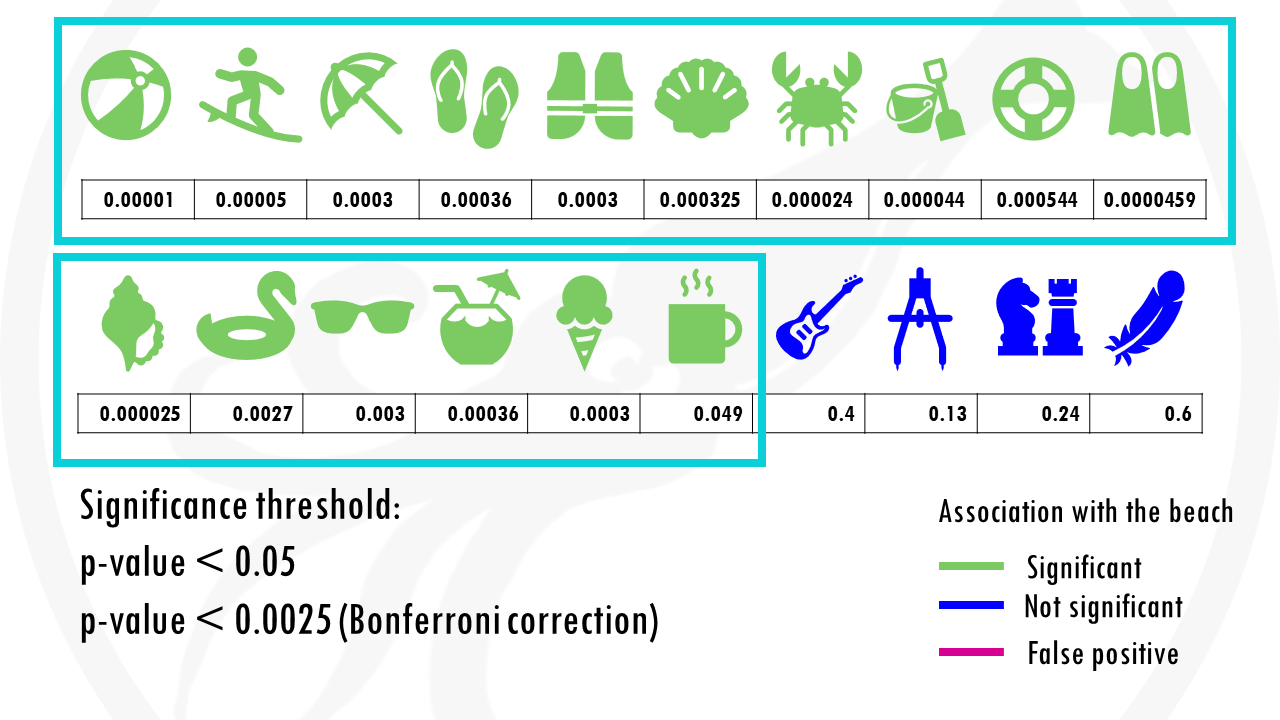
If we use our first method to correct for multiple testing, the Bonferroni correction, we would have to use a p value of 0.00205.
This means that the cup of coffee would no longer be considered associated with the beach.
Nice! But at the same time… we are losing some objects that would be interesting for us. For example, the floatie and the sunglasses are now false negatives.

Is there not another way of solving the problem of multiple testing?
Of course there is!
The Bonferroni correction lowers the p-value for all objects.
But what if we could control what happens to significant samples only?
The False Discovery Rate (FDR)
The False discovery rate, or FDR, is the proportion of false positives among all significant results.
False positives, for example, are genes that are not statistically significant, so they are not interesting for us, but just by chance they got a p-value lower than 0.05.

In our example there is 1 false positive, the coffee, amongst 15 significant results, so the FDR is 1/15 so 6.7%.
What we want to do, is bring this number down. So within our significant results, reduce the number of falsely significant results.

The first method proposed to control the FDR was Benjamini – Hochberg procedure. Soon afterwards, the q-value was introduced as a more powerful approach to controlling the FDR.
In both cases, we get a new list of corrected or adjusted p-values for each test.
A p-value of 0.05 means that 5% of all tests will result in false positives.
A p-adjusted of 0.05 means that 5% of significant results will result in false positives.

The False discovery rate, or FDR, is the proportion of false positives among all significant results.
Let’s go back to our example.
Now we get p-adjusted values for each of our objects.
So in this case, if we go with objects with a p-adjusted or q-value threshold of 0.05, it means we are willing to accept 0.75 (so less than 1 object) that’s classified as a beach object when it is not. So basically there will be less than 1 false positive.

Using q-values allows us to decide how many false positives we are willing to accept among all the features that we call significant. It is up to us to decide the threshold, as it depends on the type of analysis.
Using q values is particularly useful when we want to make a lot of discoveries to filter out later on, especially large scale, like in genomics.
For example, if you are doing a pilot study or exploratory analysis on genes correlated with Alzheimer’s, you want to avoid losing potential interesting genes, but you also don’t want a lot of false positives, so you can use q-values for this.
I hope this explanation gave you a clear overview of what is multiple testing and the main correction methods.
And that is the end of this tutorial!
In this post, I explained the differences between log2FC and p-value, and why in differential gene expression analysis we don't always get both high log2FC and low p-value. Hope you found it useful!
Before you go, you might want to check:
Squidtastic!
You made it till the end! Hope you found this post useful.
If you have any questions, or if there are any more topics you would like to see here, leave me a comment down below.
Otherwise, have a very nice day and... see you in the next one!

How were the q-values computed?
Hi! Thanks so much for your comment. Q-values control the False Discovery Rate (FDR) and are computed from p-values:
1. Sort p-values in ascending order: p₁ ≤ p₂ ≤ … ≤ pₘ
2. For each p-value pᵢ, compute: q(pᵢ) = min{FDR × m/i, 1}
3. Enforce monotonicity by working backwards
This is the Benjamini-Hochberg procedure, where m is the total number of tests and FDR is your desired false discovery rate.
This is quite a nice explanation, in case you want to do further reading! https://www.nonlinear.com/progenesis/qi/v2.0/faq/pq-values.aspx