Beta diversity: Jaccard, Bray-Curtis, NMDS, PCoA and PERMANOVA

If you’ve ever hiked from a dense forest into an open grassland, you’ve probably noticed how dramatically the plants, insects, and animals can change within just a few miles. This variation in species composition from one place to another is what ecologists call beta diversity — a key concept in understanding how life is distributed across landscapes.

While alpha diversity measures the richness of species within a single site, and gamma diversity captures total diversity across a larger region, beta diversity sits in between. It tells us how different communities are from each other. Are two wetlands home to mostly the same bird species? Or does each host a completely distinct community? Beta diversity gives us the tools to quantify those differences.

In this post, we’ll break down what beta diversity really means and how it’s measured.

So if you are ready… let’s dive in!

What is beta diversity?

In my previous blogposts, we discussed alpha diversity metrics like the Shannon, Simpson, Gini , Chao1 indices as well as Hill numbers. Alpha diversity metrics are just ways to measure the diversity in a single site or community.

Beta diversity metrics, on the other hand, allow us to compare communities. You can compare them between locations (How much does the community change if I walk 1km away?), or times (how much does the B-cell repertoire change before and after infection? Or a forest before or after a fire?). It tells you how much the “list of species” changes as you move from one community to another.

I will also introduce the concept of gamma diversity, which is the total number of species across the entire region, a region being a group of communities. So, for example, we can consider the gamma diversity of a whole park. The park has different communities, for example, it has several ponds. So we can consider the alpha diversity of each community or pond individually, we can check how many species are shared between two communities using beta diversity metrics, or we can consider the entire park to get gamma diversity.

Diversity metrics can also be applied to the antibody repertoire in individuals. Our gamma diversity would be the BCR repertoire of a cohort of patients, each patient being a community. We can look at the diversity within a single patient (alpha) or we can look at the shared and distinct clonotypes between patients (beta).

In a nutshell:

Alpha Diversity — measures diversity within a site or community. Think of it as local diversity. Alpha diversity can be measured simply as species richness (total number of species), or using indices like Shannon or Simpson that also account for evenness (how evenly individuals are distributed among species). In all cases, it refers to the number of species found in a single habitat or sampling area. 

Gamma diversity is the total diversity across a larger landscape or region that includes multiple habitats or communities. Gamma diversity combines:

• The diversity within individual sites

• The differences between those sites

Beta Diversity measures the diversity between sites – difference in species composition between habitats or communities. In simple terms, beta diversity captures species turnover across space.

• High beta diversity means communities are very different from one another
• Low beta diversity means communities are quite similar

How to interpret beta diversity with an example

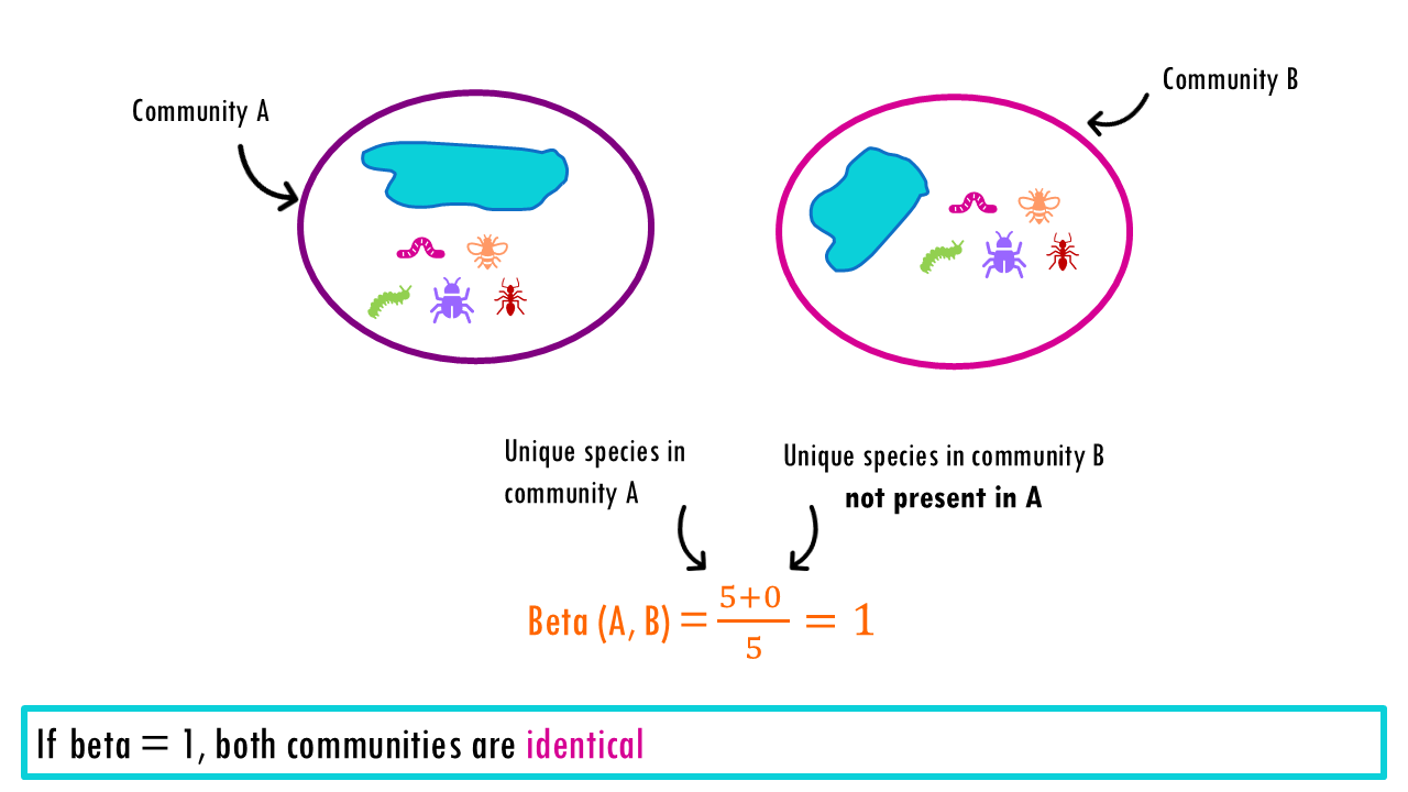
The Beta Diversity represents the number of “pure” (distinct) communities in a region.

• If we compare ponds 1 and 2, we have Beta = 5/5 = 1. When beta = 1, it means that our communities or sample sites are identical (they act like 1 single community). These two ponds contain the exact same number of species so there is no change between them. Beta = 1 tells us that this region is essentially just one single community Moving from Pond 1 to Pond 2 gives you nothing new.
• If we compare Pond 1 and 3, we get beta = 5 + 5 / 10 = 2. This “2” is telling you that the region contains exactly two completely different communities. To see everything the park has to offer, you have to visit two distinct sites because there is zero overlap.

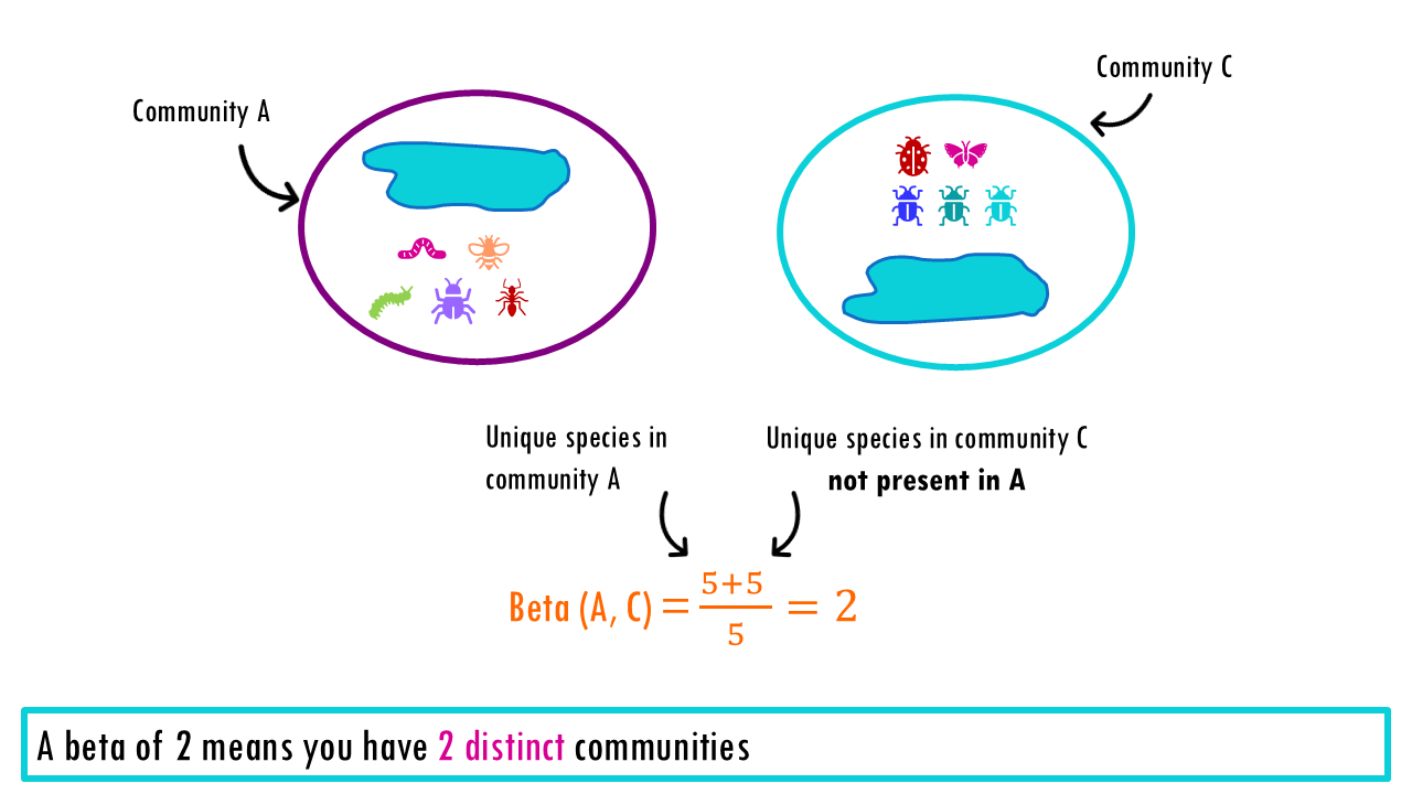
A value of beta that sits somewhere in the middle between 1 and 2, means there is some overlap. The higher the value of beta, the more distinct both communities are.

Global beta diversity

We know how to calculate the beta diversity of two communities, but what about the beta diversity of the entire region? The beta diversity of a group of communities tells us how many distinct communities we have overall. For example, a country might have 8 national parks, but if they all have very similar species, the beta diversity will be lower than that of a country with 2 national parks that are very different.

The beta diversity of the entire park would be calculated as follows:

Step 1: Calculate Average Alpha

Alpha is the diversity of an average site. We saw how there are different ways to calculate alpha diversity, here to simplify I will just use the richness or total number of distinct species because that way we can just calculate a simple average.

Step 2: Calculate Gamma

Gamma is the total number of unique species in the entire region. Since Ponds 1 and 2 are identical, they only contribute 10 species. Pond 3 adds 10 new species.

Step 3: Calculate Beta

Using Whittaker’s multiplicative formula:

Gamma = Alpha x Beta

Even though we have 3 ponds, our Beta diversity is 2. This tells us that your region effectively contains two unique biological “sets” or communities or ponds. The math “ignores” the fact that we have a duplicate pond because that duplicate doesn’t add any new diversity to the landscape, so it’s as if we had 2 ponds.

The beta diversity can also be interpreted as the region is twice as diverse as our average pond. If we zoom in to one site, we’ll see an average of 5 different species, if we zoom out, we see 10 different species, so the regional diversity, is 2 times larger than what we saw at the local level.

As a rule, if beta is less than the number of sites (in this case beta = 2 but we have 3 sites), then it means that overlap exists between sites.

We’ve talked about Whittaker’s beta which is a Global Measure of diversity. It looks at your entire dataset (all ponds in a region, all samples in a patient cohort) at once and gives you a single number representing the total “turnover” across the whole landscape.

But maybe we’re just interested in calculating the beta diversity between two communities. For example, to compare the B cell repertoire between two patients. For that we can use pairwise measures of beta diversity that compare exactly two sites at a time.

Pairwise beta diversity metrics

Pairwise measures of beta diversity that compare exactly two sites at a time.

To compare samples, we compute dissimilarities:

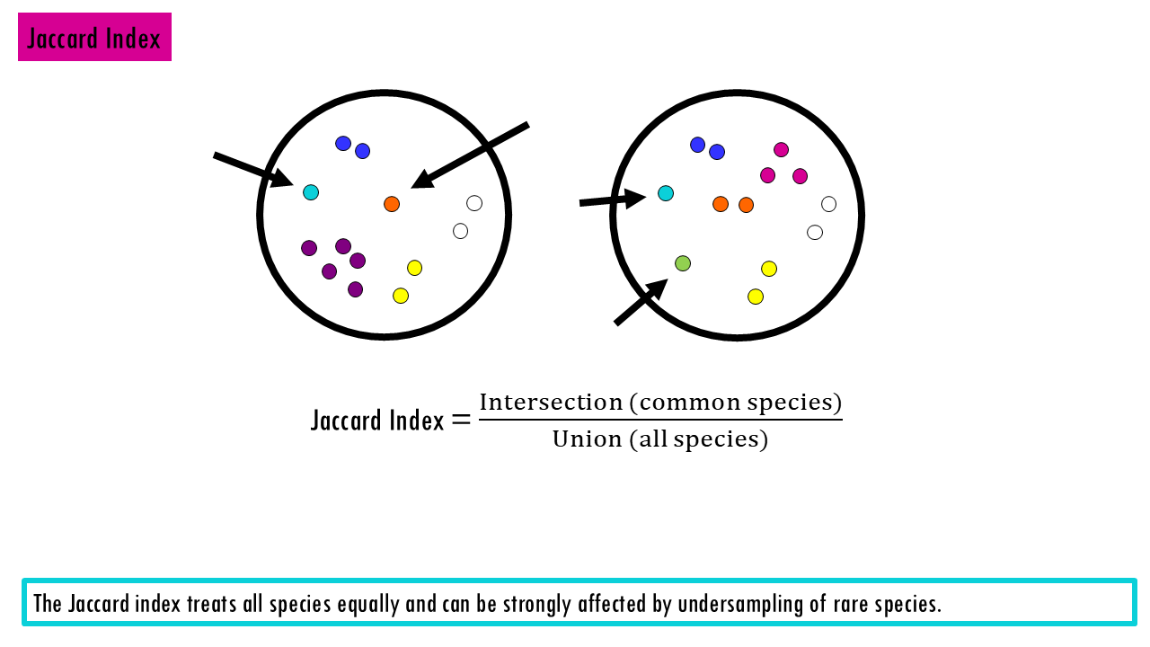
• Presence/absence metrics (Jaccard, Sørensen) treat all species equally and can be strongly affected by undersampling of rare species.
• Abundance‑based metrics (Bray–Curtis, Morisita, etc.) incorporate relative abundances and can be more robust to undersampling of rare species but emphasize common species differently. 
• Distances feed ordination (PCoA / NMDS) and statistical tests (PERMANOVA) can also be used see if your Beta diversity differences are statistically significant between groups.

Presence/Absence Metrics (Binary)

These use only whether species are present or absent (not abundance). These metrics only care if a species is there or not (0 or 1). They are great for studying biogeography or when your data quality doesn’t allow for accurate counting.

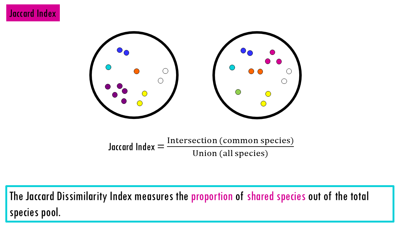
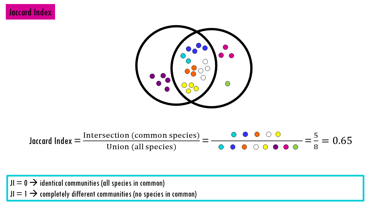
Jaccard Dissimilarity Index: Measures the proportion of not shared species out of the total species pool. “Of all the species found in both places, what percentage do they have in common?” 

• 0 = identical communities
• 1 = completely different

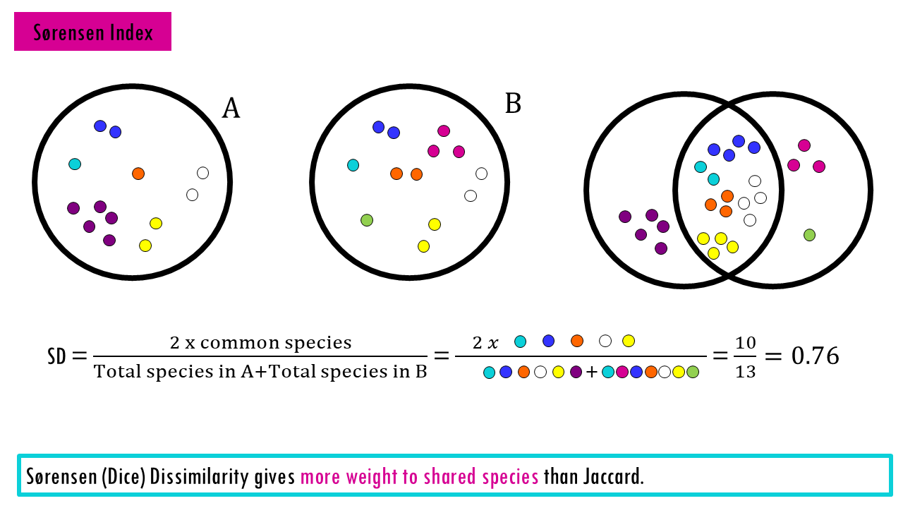
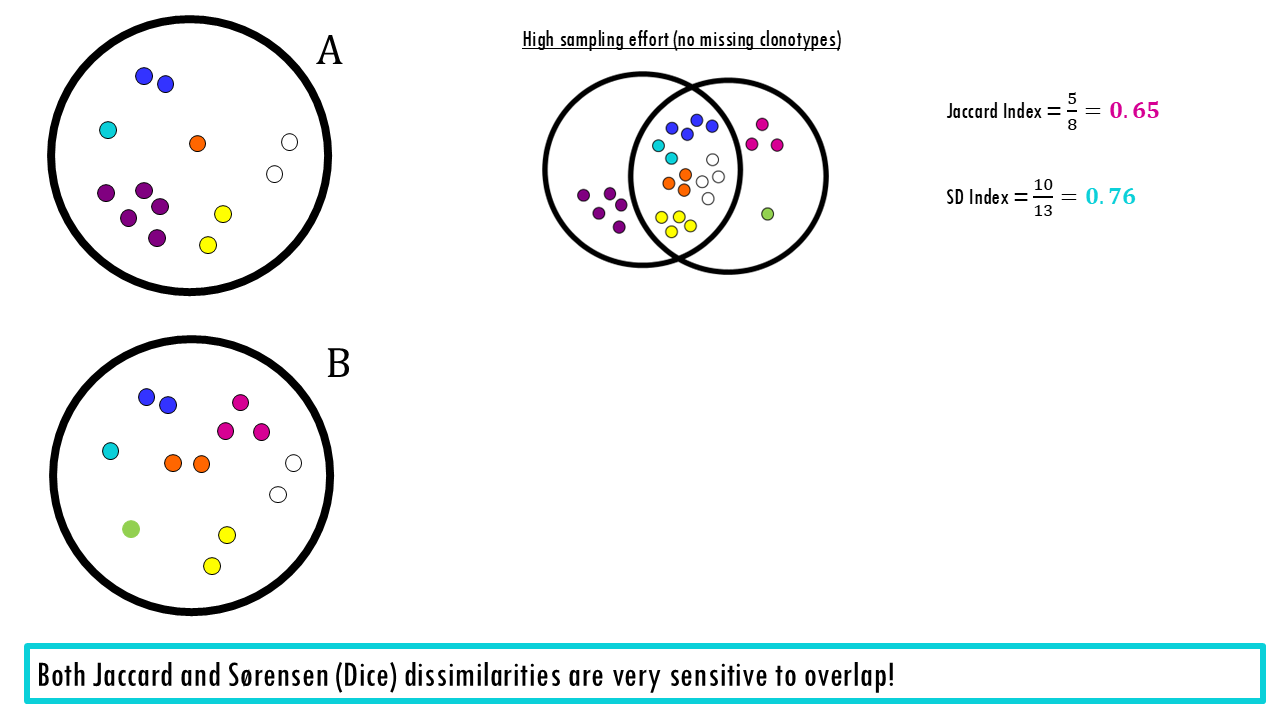
Sørensen (Dice) Dissimilarity gives more weight to shared species than Jaccard. It’s often preferred in ecological studies because it’s slightly more sensitive to overlap.

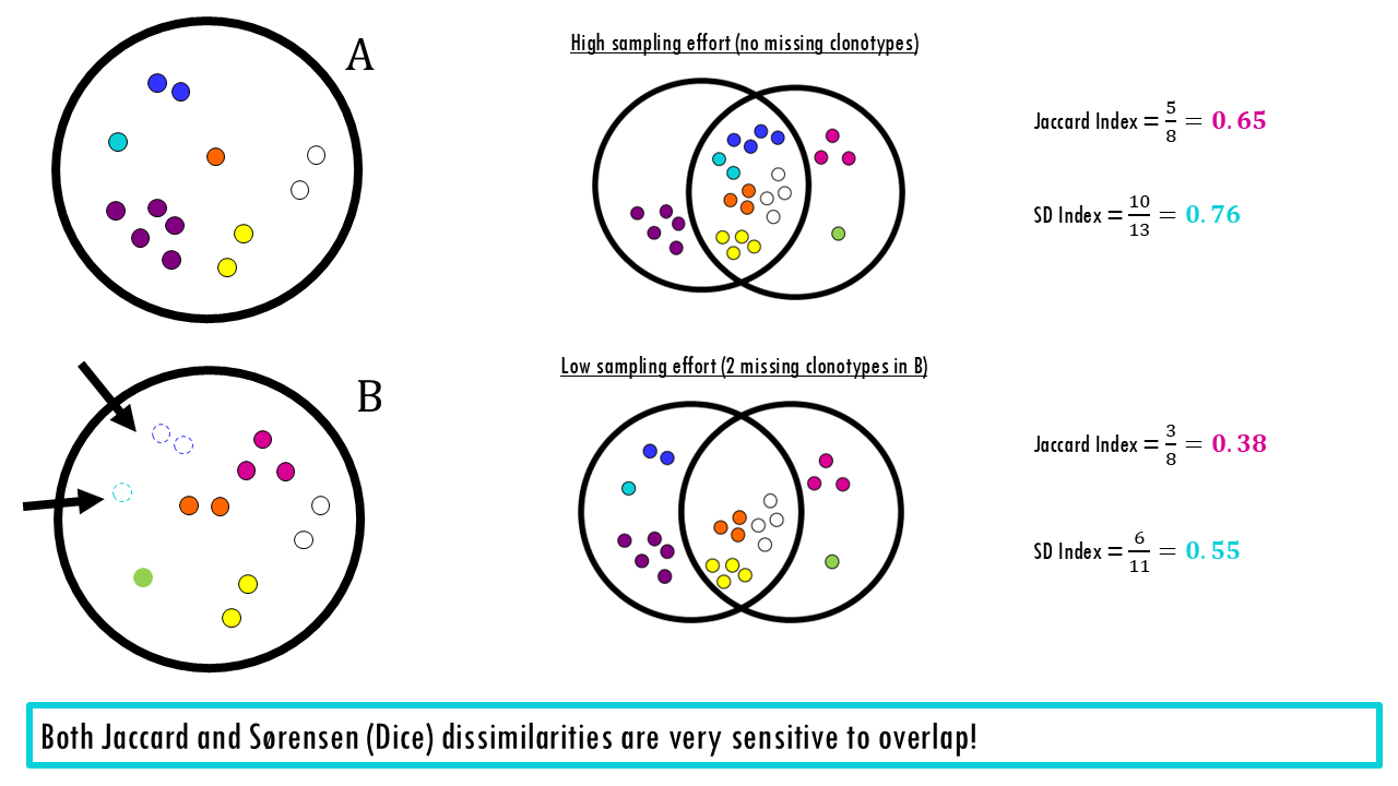
Remember that because these treat a single sighting of a rare orchid the same as 10,000 blades of grass, they are highly sensitive to “noise.” If you miss a rare species due to sampling effort, your similarity score drops significantly.

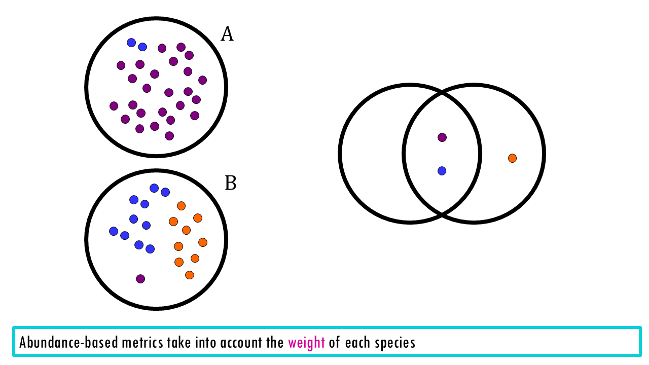
Abundance-Based Metrics (Quantitative)

These look at the “weight” of each species. If Sample A has 100 lions and Sample B has 1 lion, these metrics will show a massive difference, whereas a presence/absence metric would say they are “the same” (both have lions).

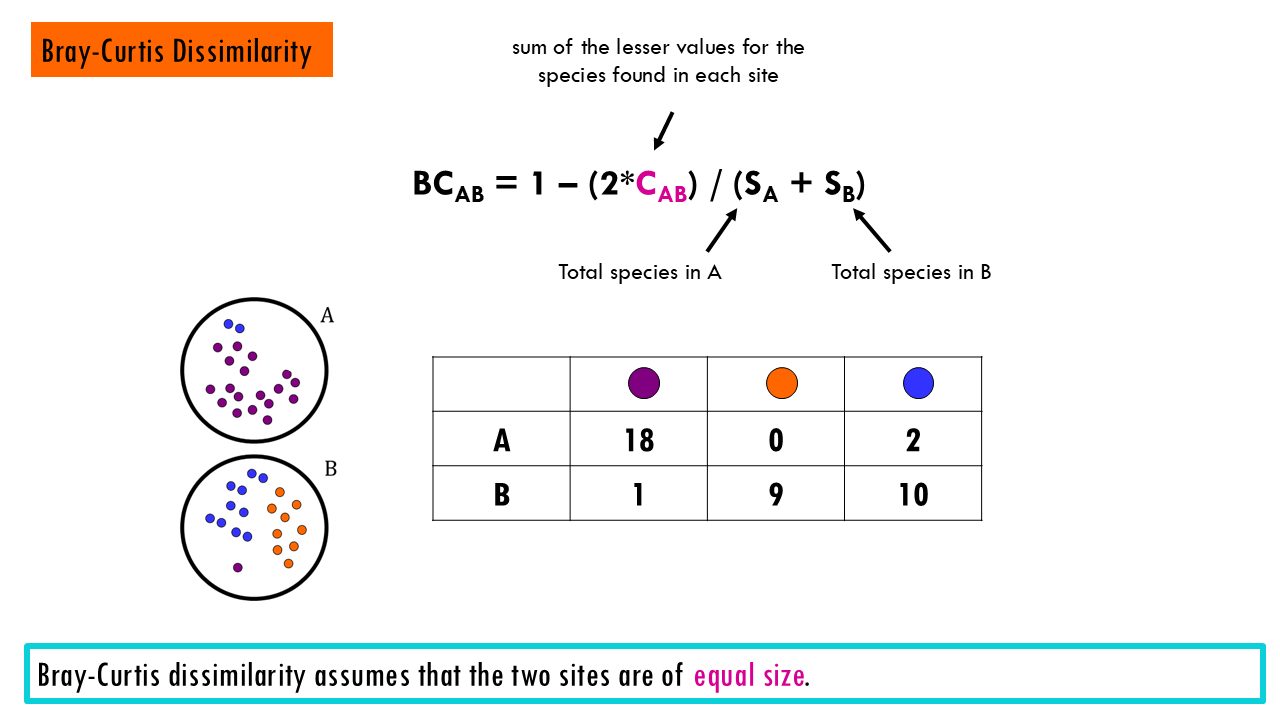
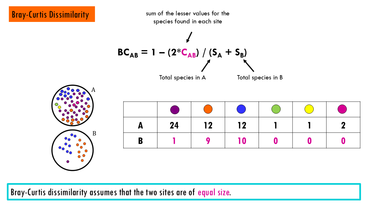
Bray-Curtis Dissimilarity is one of the most widely used metrics in ecology. It compares abundance differences between sites.

• 0 (identical)
• 1 (completely different)

Morisita-Horn: This is less sensitive to total sample size (sampling effort) and more focused on the relative proportions. It’s often used when you have uneven sampling depths between sites.

Visualizing and Testing: Ordination & PERMANOVA

Once you’ve calculated pairwise beta diversity (e.g., Jaccard or Bray–Curtis distances), we will have a a distance matrix (essentially a big table showing how different every sample is from every other sample),

The next step is usually:

1. Visualize patterns in community composition
2. Statistically test whether groups differ

That’s where ordination and PERMANOVA come in.

Ordination: Visualizing Multivariate Community Data

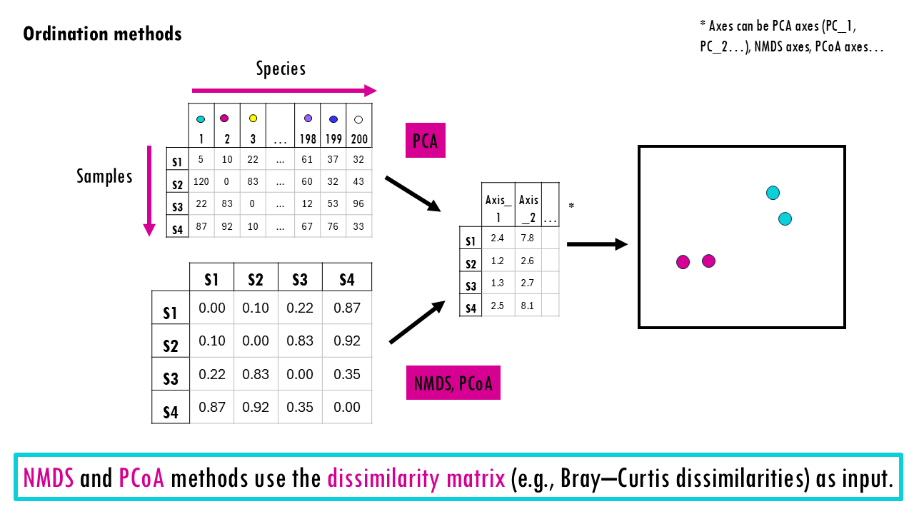
Community data are multivariate — each species is a dimension. If you have 200 species, that’s 200-dimensional space. Ordination methods reduce this complexity to 2–3 dimensions so we can visualize patterns. They use your distance matrix (e.g., Bray–Curtis dissimilarities) as input.

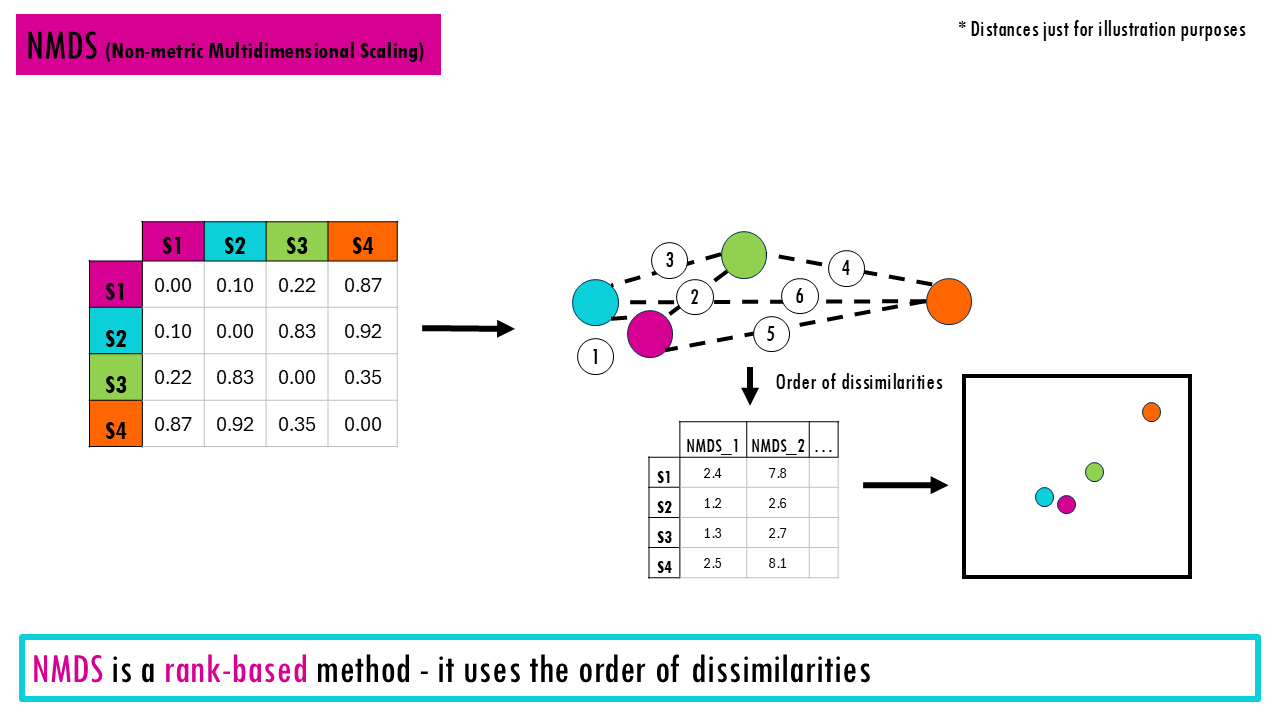
• NMDS (Non-metric Multidimensional Scaling) is a rank-based method. This means it uses the order of dissimilarities, not raw values. It’s very common in ecology and works well with Bray-Curtis. The key idea here is that sites that are compositionally similar appear closer together in ordination space. Check out this blogpost for an NMDS tutorial in R.
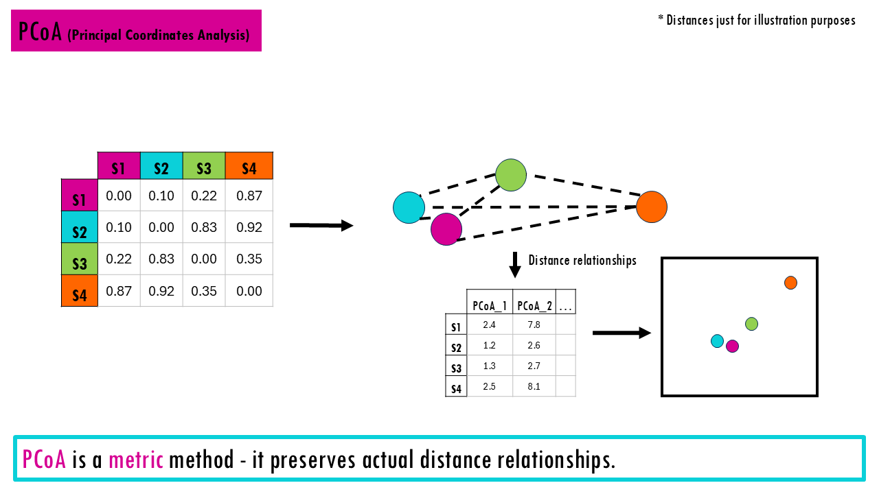
• PCoA (Principal Coordinates Analysis) is a metric method, meaning it preserves actual distance relationships. It works with many distance measures and it is especially useful when you want eigenvalues and variance explained.
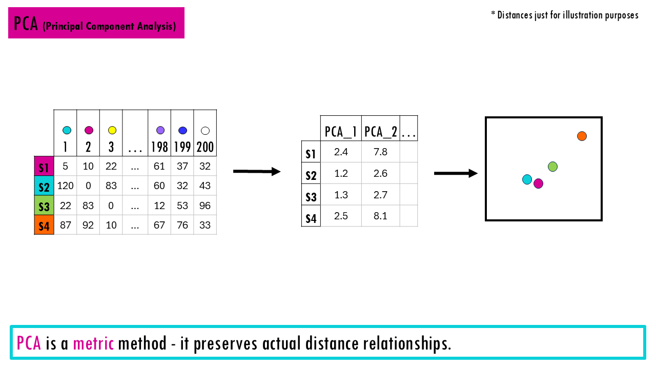
• PCA (Principal Component Analysis). Note that is is not the same as PCoA! It’s based on raw abundance data. The big difference is that it assumes Euclidean distances and is more sensitive to scaling, so it is less ideal for zero-heavy ecological datasets and non-Euclidean dissimilarities (e.g., Bray–Curtis). You can read more about PCA in my other blogpost by clicking here!

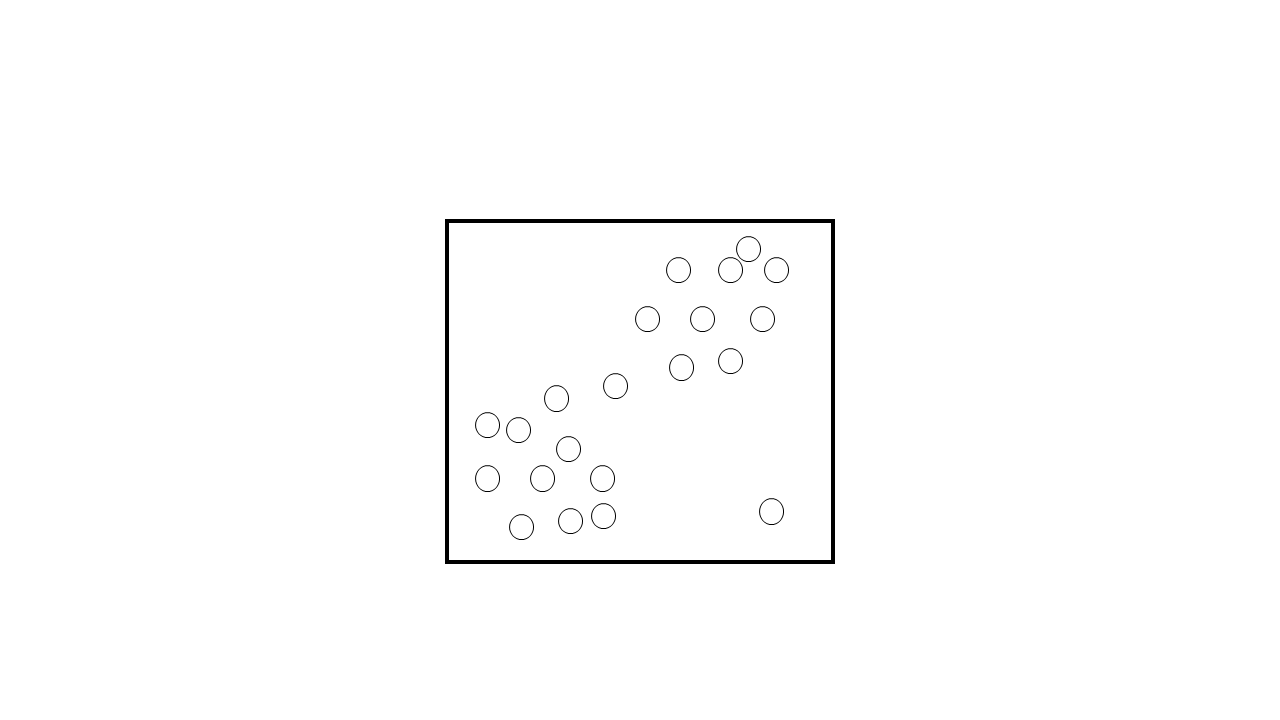
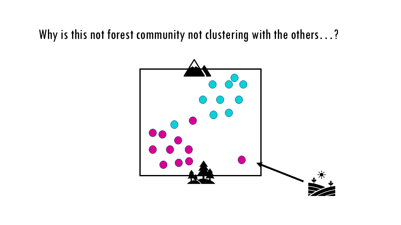
How to interpret an ordination plot?

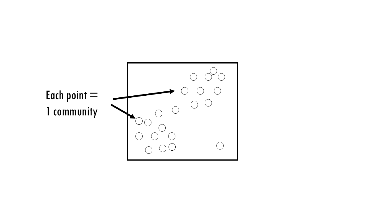
Essentially, all these plots (NMDS, PCoA, PCA) have a similar structure.

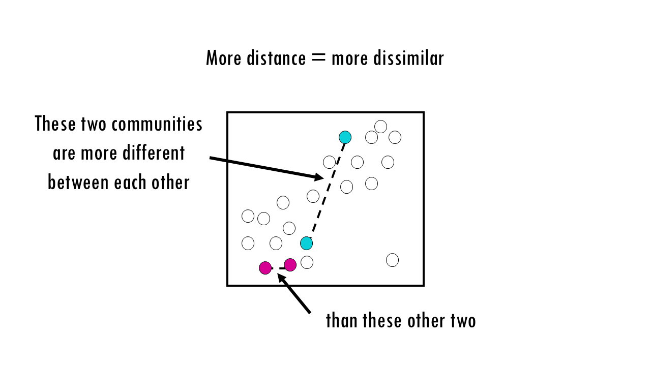
• Each point is one site
• The distance between points is compositional dissimilarity – the further away two points / communities are, the more dissimilar they are.
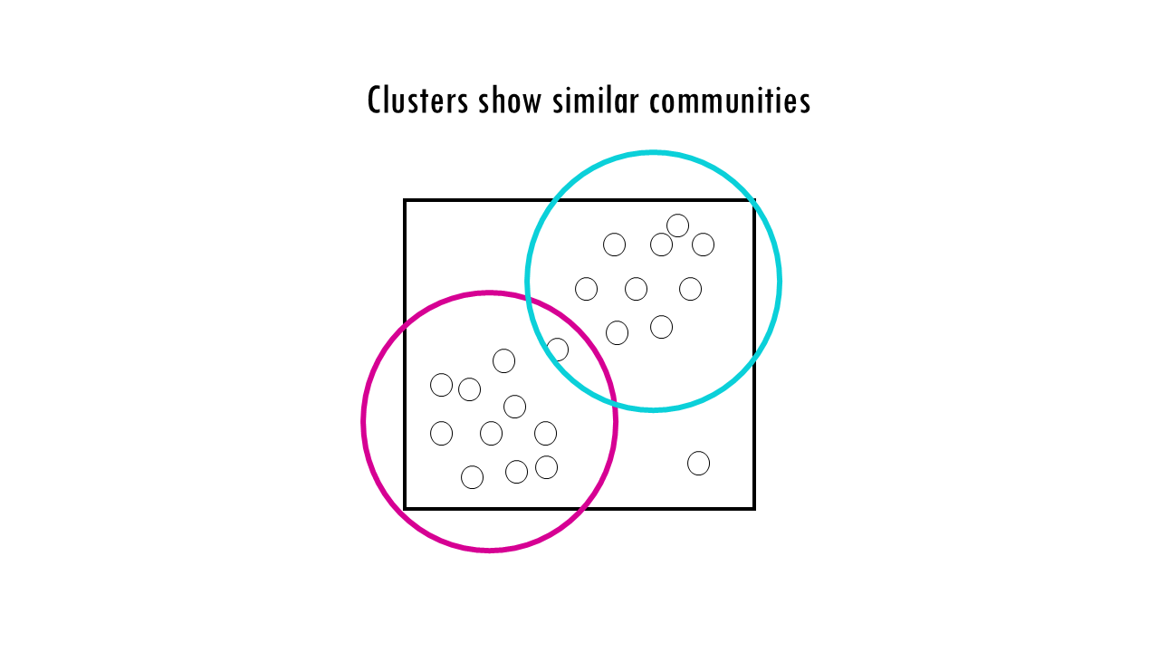
• Clusters show similar communities

Ordination is exploratory — it helps you see patterns, but doesn’t formally test them.

PERMANOVA: Testing Group Differences

PERMANOVA stands for Permutational Multivariate Analysis of Variance. It basically tries to answer “Are these groups of communities actually different from each other?”

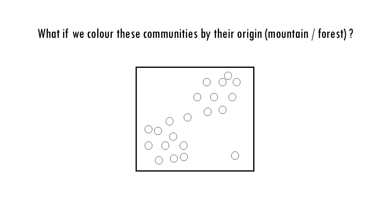
PERMANOVA tests whether community composition differs between predefined groups (e.g., treatment vs control, forest vs grassland).

So, how does PERMANOVA work?

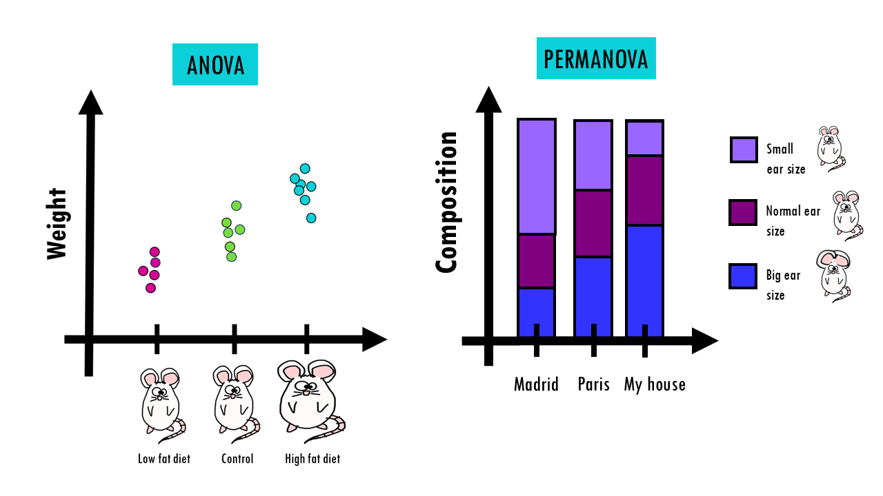
You might be already familiar with ANOVA, which is a statistical test to compare a metric (for example, height or weight) between 3 or more groups (if not you can read this other blogpost!). But while regular ANOVA compares means of numbers, PERMANOVA compares whole communities using a distance matrix (like Bray–Curtis dissimilarities).

So instead of comparing averages of one variable, it compares multivariate differences between groups.

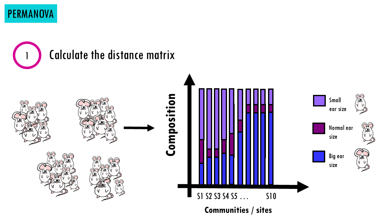
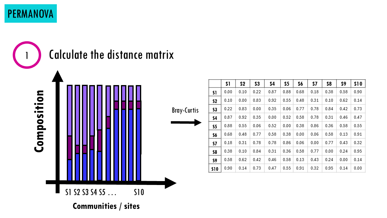
How does it work?

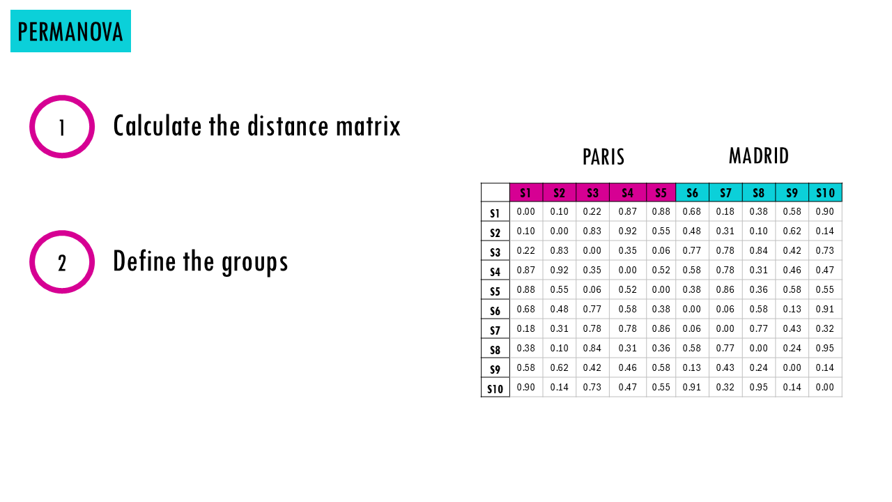
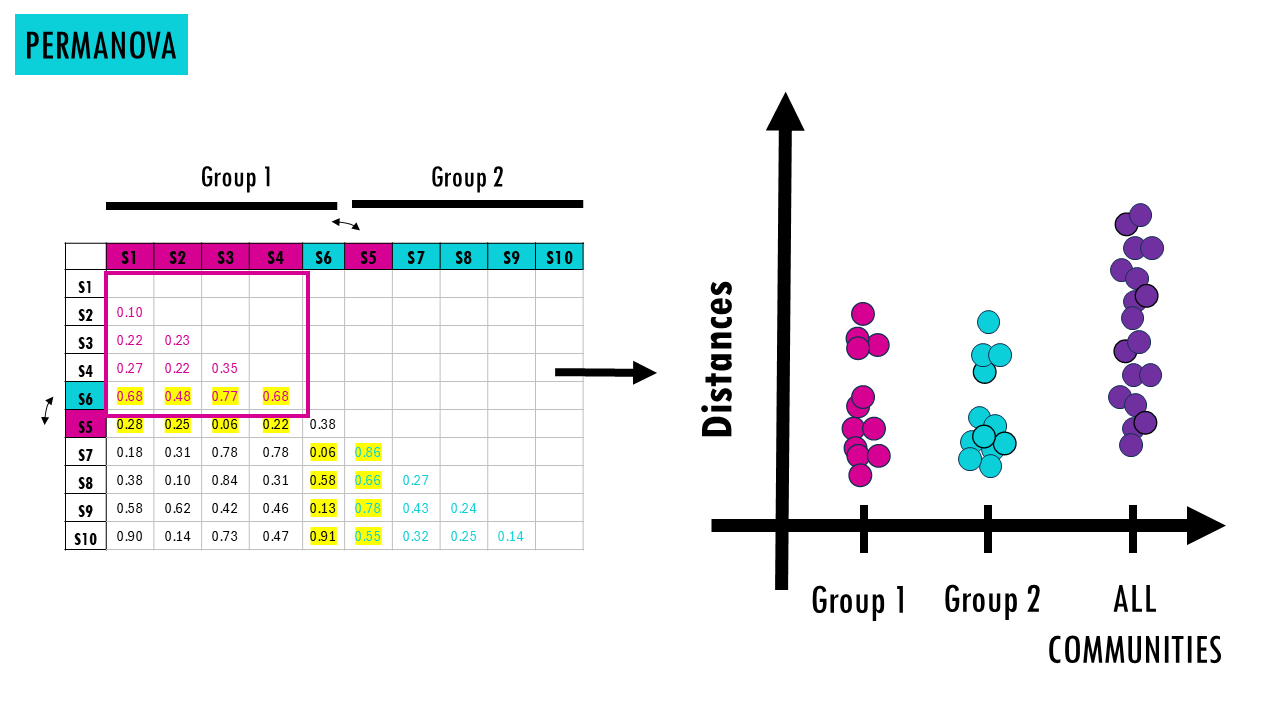
1. First, we calculate the distance matrix (e.g., Bray–Curtis). Now we have a table of distances between all sites which tells us how different each pair of sites is.
2. Then we define the groups (i.e., forest vs grassland, control vs treatment, year 1 vs year 2, before or after infection… you get it!). 
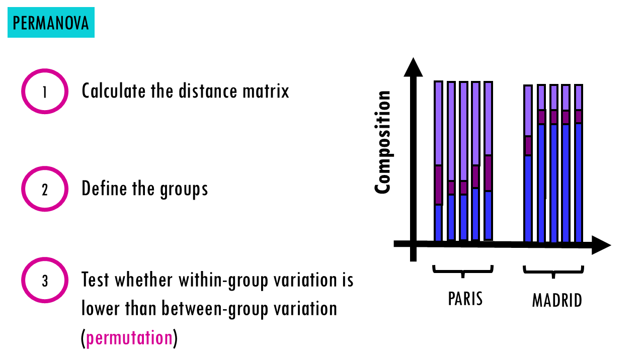
3. Now, PERMANOVA uses permutation to test if sites within the same group more similar to each other than to sites in other groups. If yes, it means groups statistically differ. 

Wait a minute, permutation? 

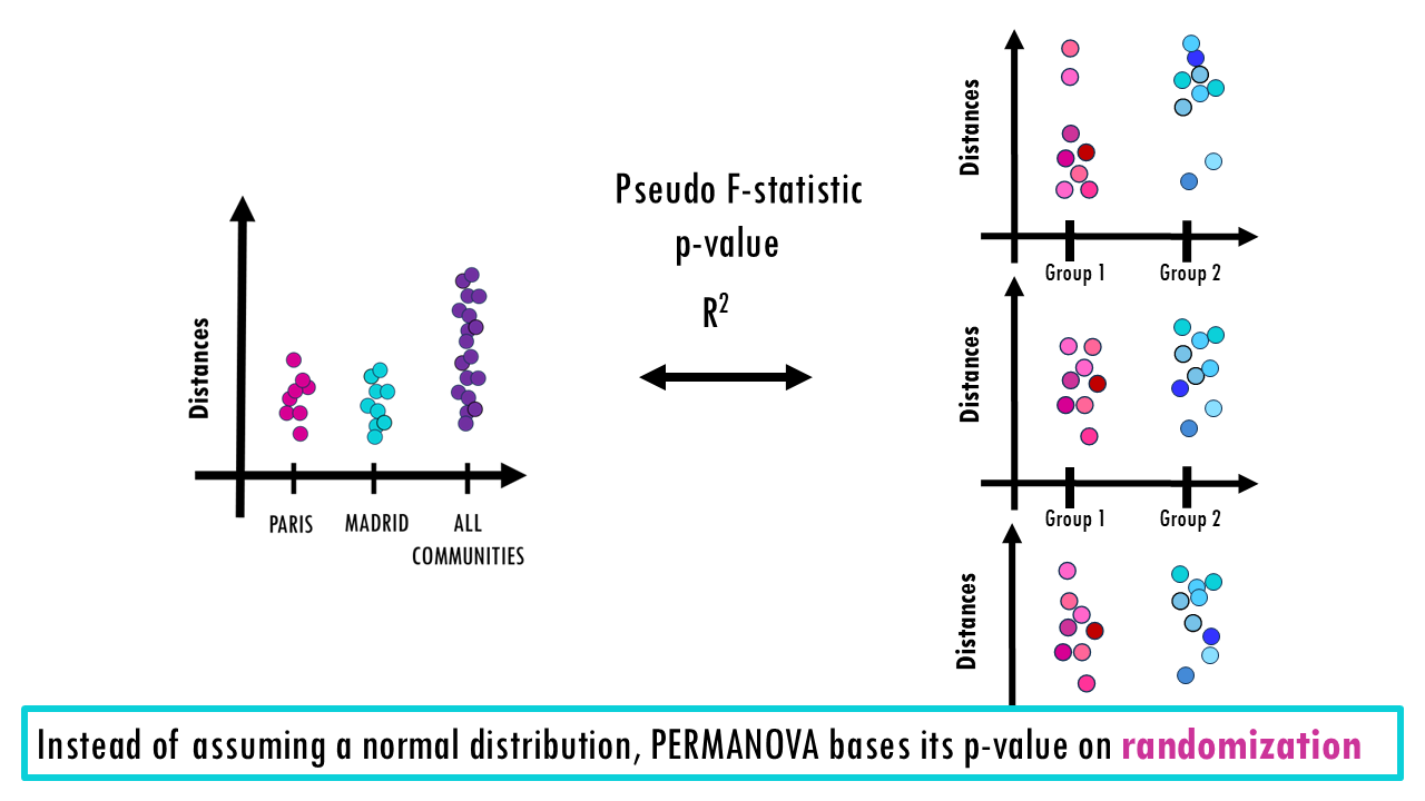
Instead of assuming normal data, PERMANOVA:

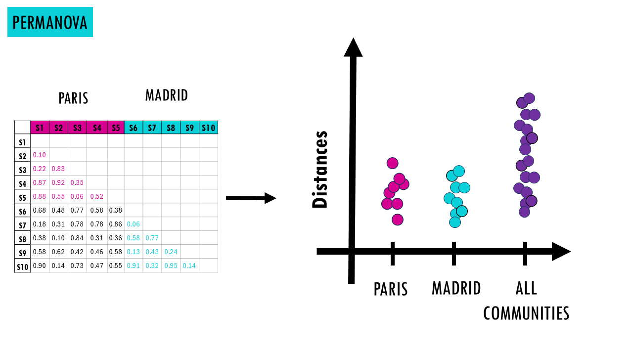
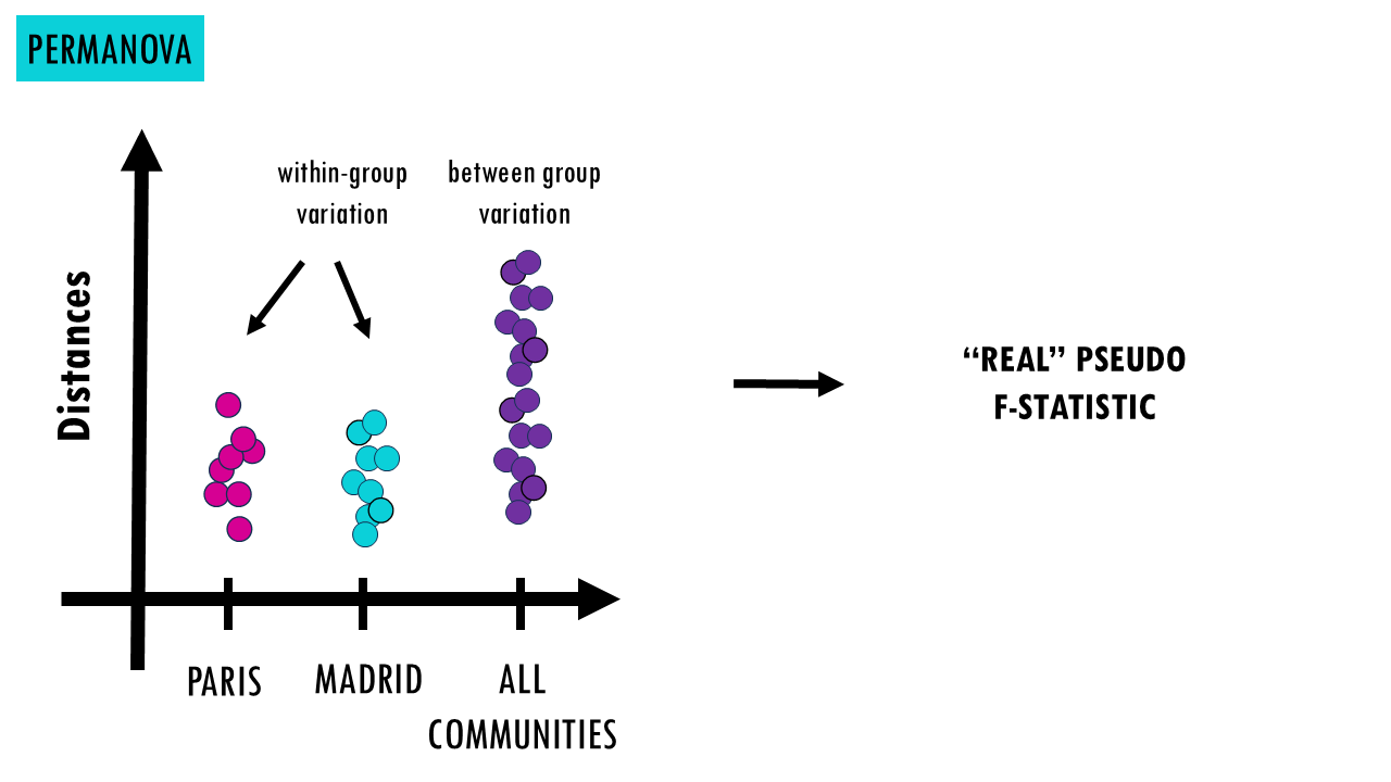
1. Calculates the real test statistic (how different your groups actually are in your real dataset). You can check my ANOVA blogpost to learn more, but it essentially divides between-group variation by within-group variation.
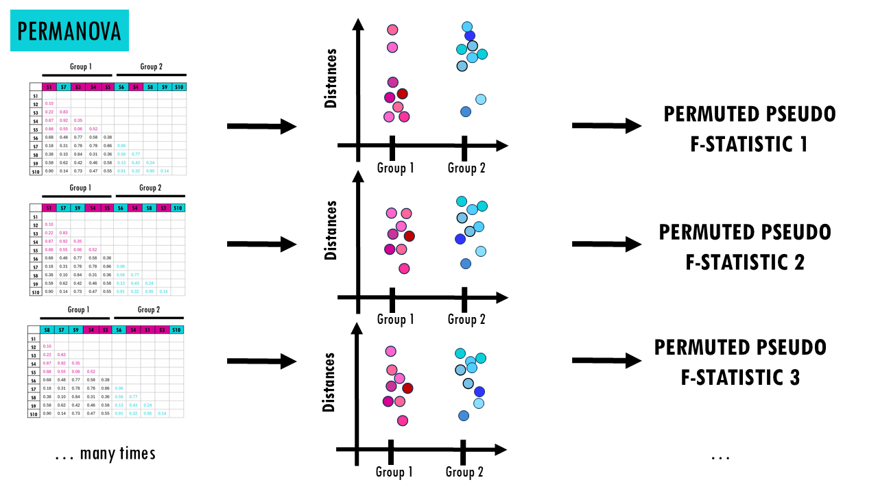
2. Randomly shuffles group labels many times
3. Recalculates the statistic each time
4. Sees how extreme your real result is

If your observed difference is larger than most random shuffles it means there is a significant difference. So the p-value is based on randomization, not mathematical distribution assumptions.

How to interpret PERMANOVA results?

A PERMANOVA test will give you:

• Pseudo-F statistic (effect size proxy)

• R² value (variance explained)

• p-value (based on permutations)

For example, if we run a PERMANOVA test between two habitats and get significant differences in composition between them (R² = 0.21, p = 0.001); it means the grouping variable – for example, the habitat, grassland vs forest – explains 21% of community variation, and that the effect is statistically significant (unlikely due to random chance).

Before running PERMANOVA though, make sure your groups have similar variability – PERMANOVA assumes homogeneous dispersion (similar spread within groups).

Final notes

Squidtastic!

In this blogpost we covered beta diversity metrics, including global diversity metrics (gamma divided by alpha) as well as pairwise diversity metrics. We’ve briefly explained metrics like Jaccard or Sorensen, as well as ordination (PCoA, NMDS…) and PERMANOVA. If you would like to learn how to implement any of these methods in R, let me know in the comments below!

Want to know more?

Additional resources

If you would like to know more about diversity metrics, check out:

• Roswell et al., “A conceptual guide to measuring species diversity” — Hill numbers & coverage (practical guidance).
• Barwell, Isaac & Kunin (2015), “Measuring β‑diversity with abundance data” — evaluation and properties of β metrics.
• Jost L., “Entropy and diversity” (Oikos, 2006) — why convert entropies to effective numbers; Hill numbers & replication property.
• Carpentries / metagenomics alpha–beta R tutorial — short instructional material and plotting examples.
• NMDS –  Applied Multivariate Statistics in R

You might be interested in…

• Diversity metrics simply explained: Shannon, Simpson, Chao1
• Hill numbers 
• UMAPs simply explained
• PCA simply explained
• t-SNE simply explained

Squidtastic!

Wohoo! You made it 'til the end!

Hope you found this post useful. If you have any questions, or if there are any more topics you would like to see here, leave me a comment down below. Your feedback is really appreciated and it helps me create more useful content:)

Otherwise, have a very nice day and... see you in the next one!

Before you go, you might want to check:

Squids don't care much for coffee,

but Laura loves a hot cup in the morning!

If you like my content, you might consider buying me a coffee.

You can also leave a comment or a 'like' in my posts or Youtube channel, knowing that they're helpful really motivates me to keep going:)

Cheers and have a 'squidtastic' day!