
Introduction to time series forecasting
From predicting a crash in the stock market, to estimating the temperature and wether you’ll need an umbrella tomorrow – time series analysis is everywhere!
In this blogpost, we’ll cover what a time series is, why order matters so much, and some examples on time series models!
So if you are ready… let’s dive in!
Keep reading or click on the video to learn about time series analysis!
What is time series analysis?
This is one patient’s PSA level – a prostate cancer biomarker – tracked over two years. Notice it’s not just a number. It’s a number with a date attached, over and over again. That’s the entire idea behind a time series: data ordered in time, where the order itself carries information.
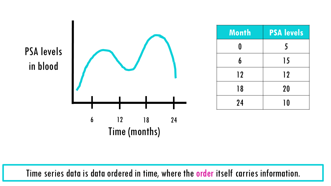
A time series is just a sequence of measurements taken at successive points in time. The key word is sequence. If you shuffled the order, you’d lose information – because in time series data, what happened yesterday often shapes what happens today.
Squidtip
A time series is just data ordered in time, where the order itself carries information.
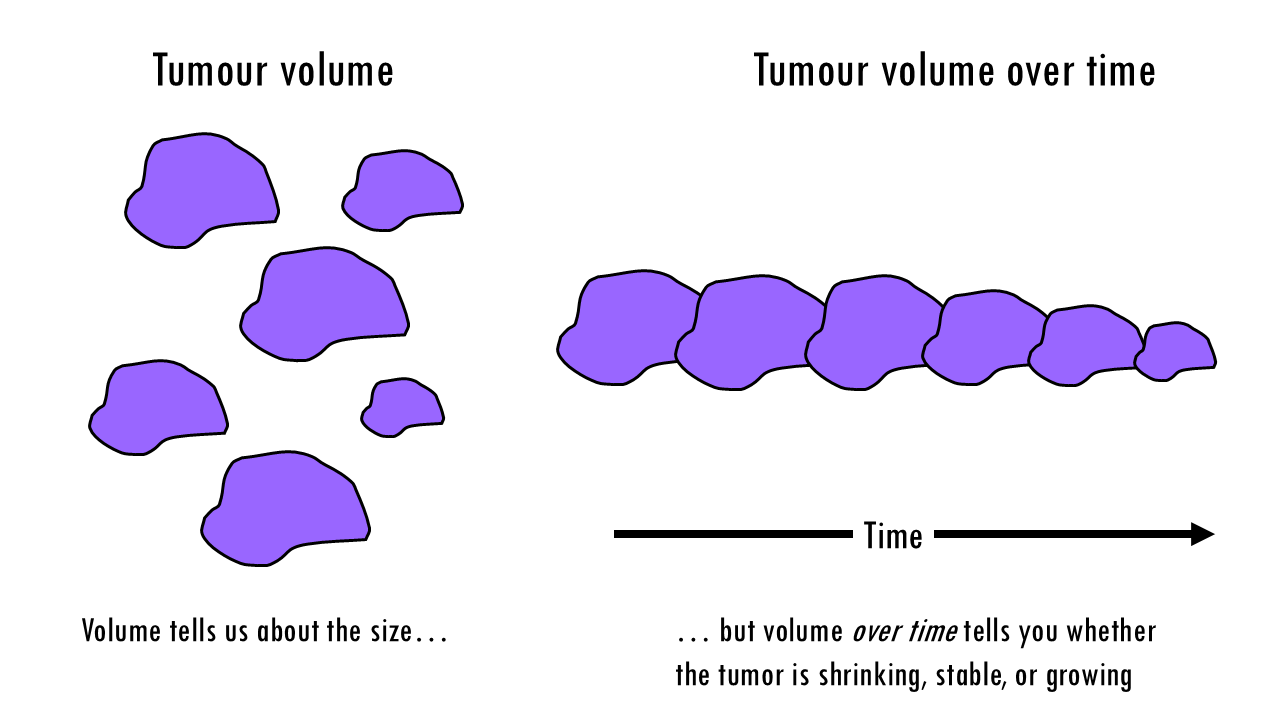
Think about tumour volume measured from CT scans every 6 weeks during chemotherapy. Volume alone tells you size. But volume over time tells you whether the tumour is shrinking, stable, or growing – which is the actual clinical question.
The Building Blocks: Trend, Seasonality, Noise
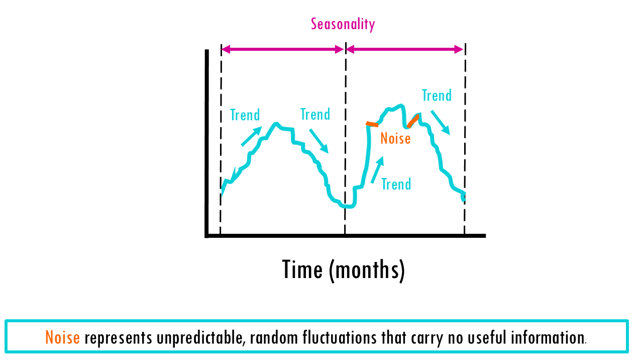
Almost every time series can be broken into three components.
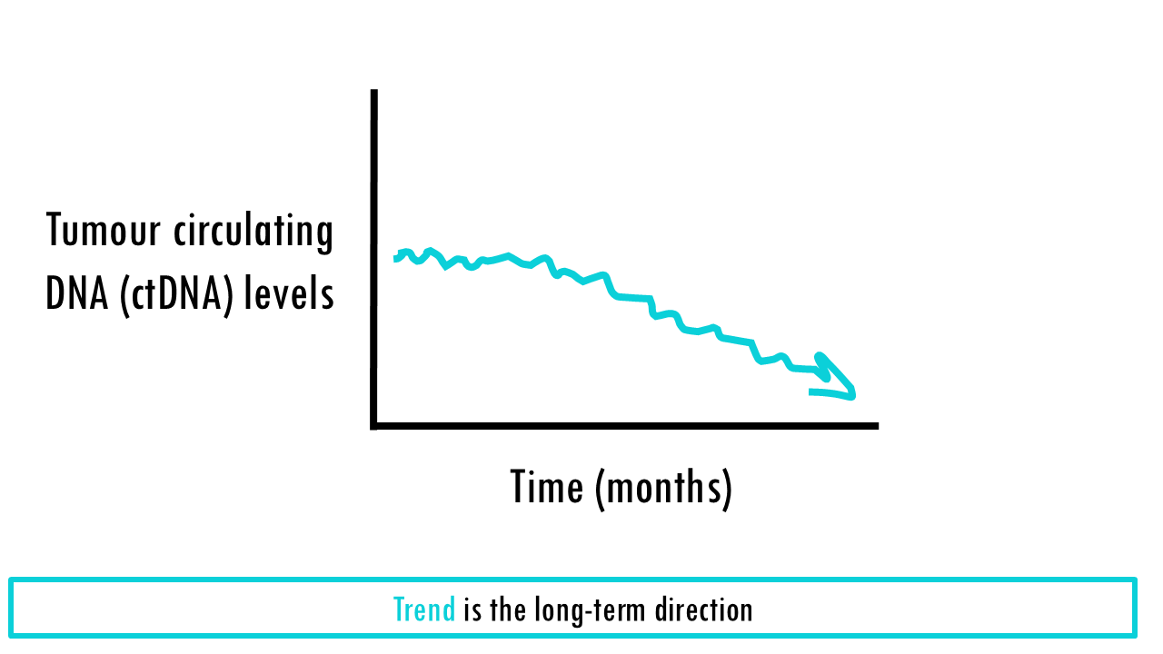
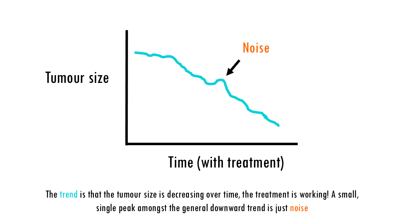
Trend – the long-term direction. In oncology: a patient’s circulating tumor DNA, or ctDNA, trending downward over months of successful treatment, or trending upward as resistance develops.
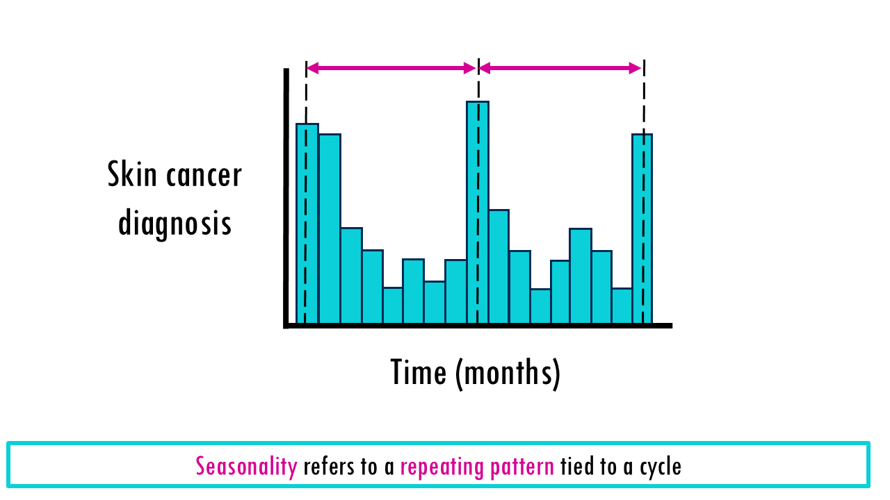
Seasonality – a repeating pattern tied to a cycle. This shows up less in individual patient biology, but it’s huge in population-level cancer data – for example, skin cancer diagnoses spiking every summer due to sun exposure patterns, or hospital biopsy volumes dipping every December.
Noise – the random wobble left over once you remove trend and seasonality. A single elevated white blood cell count the week after a cold isn’t a trend – it’s noise. This matters clinically: you don’t want to change a treatment plan because of one noisy data point. You want to know if the trend has actually shifted.
Why Order and Spacing Matter: Stationarity & Irregular Sampling
Two challenges make medical time series trickier than, say, stock prices
Stationarity
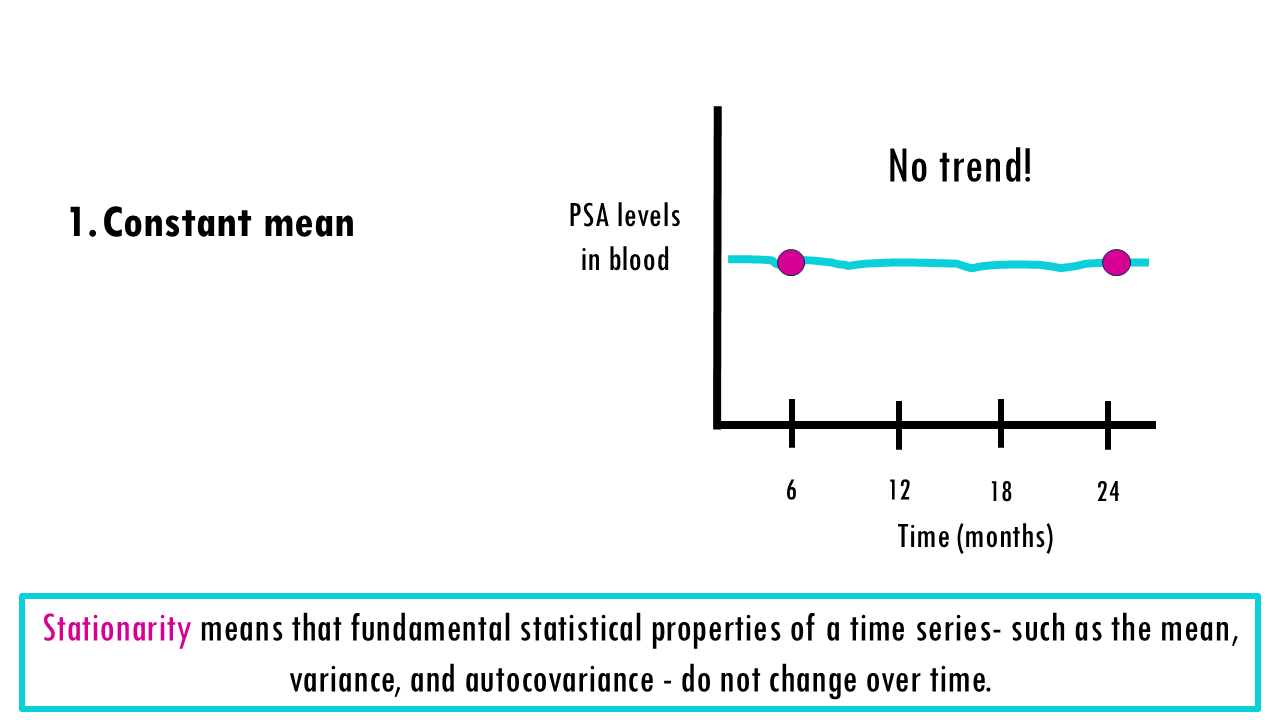
A time series is stationary if its statistical properties don’t change over time. Specifically, a stationary series has:
- Constant mean – the average value doesn’t drift up or down over time. Basically, there is no trend. If a series has a genuine trend (the mean is systematically increasing or decreasing over time rather than staying constant), then the series would be non-stationary.
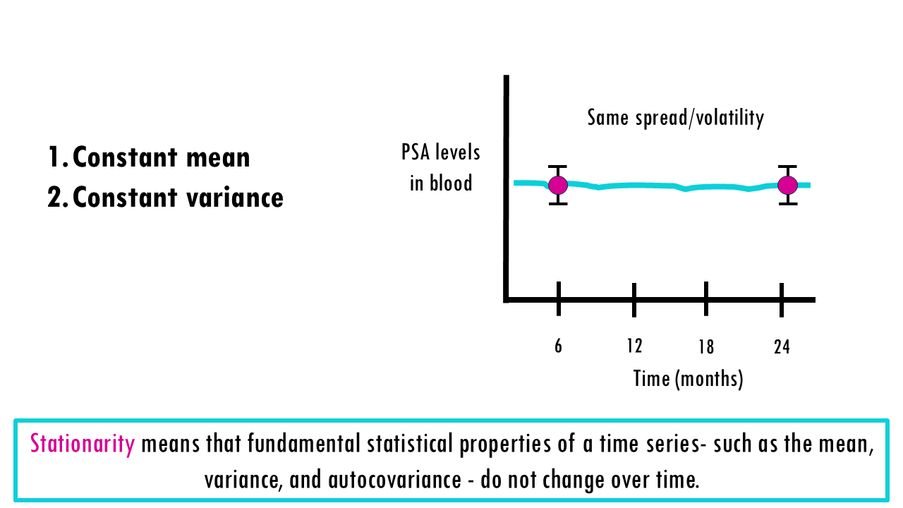
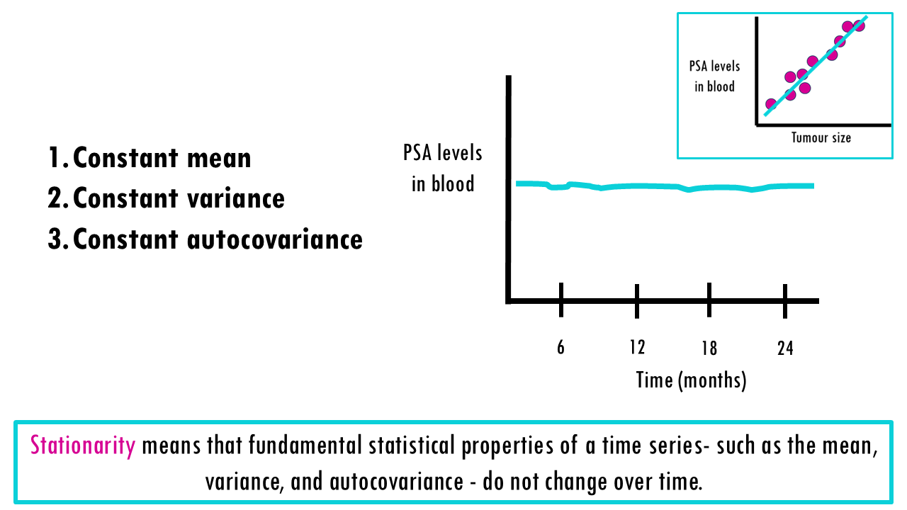
- Constant variance – the spread/volatility stays roughly the same throughout. Every biological measurement comes with some error, so we want that error to remain constant over time.
- Constant autocovariance – the correlation between values at different time lags depends only on the distance between them (the lag), not on when in time you’re looking.
Autocovariance
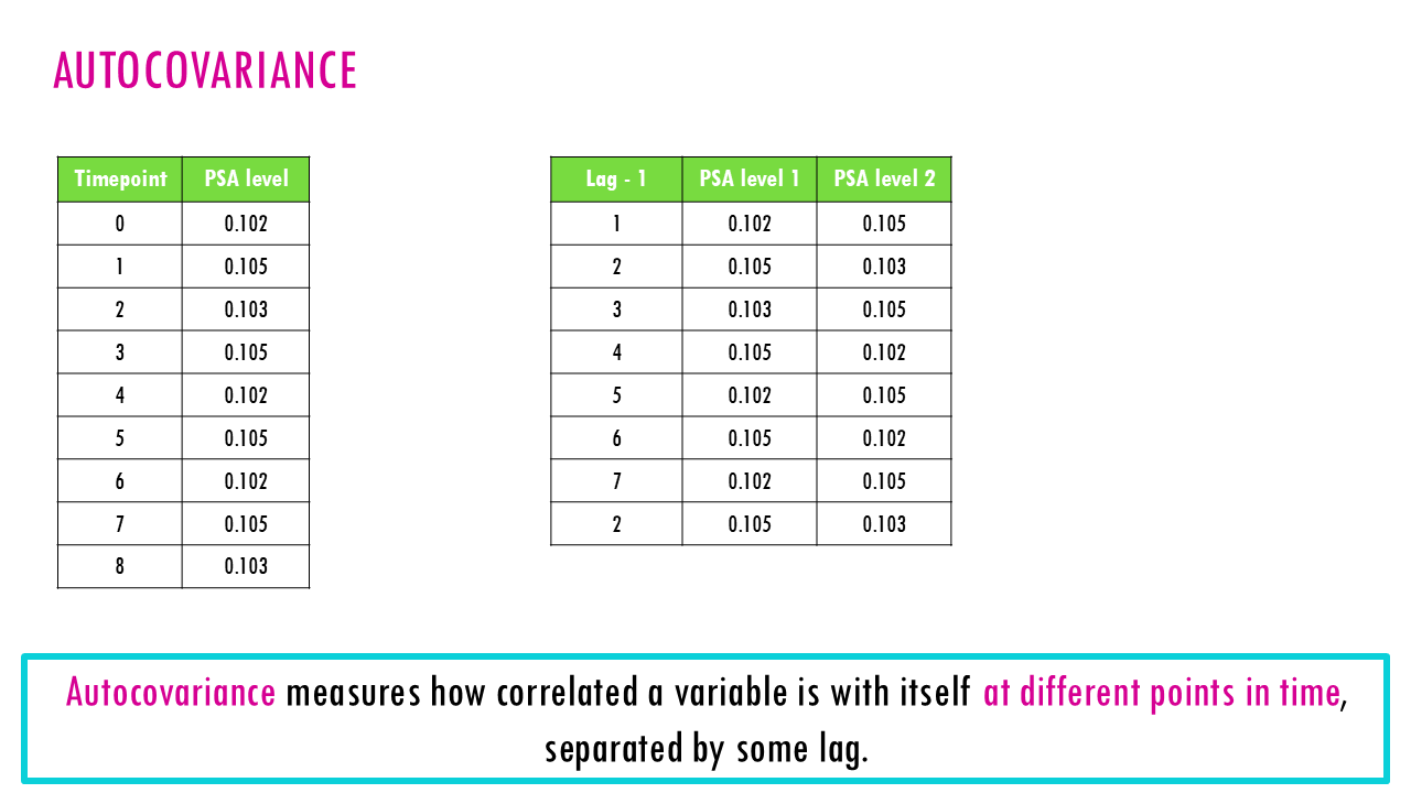
Autocovariance measures how correlated a variable is with itself at different points in time, separated by some lag.
If we go back to our PSA example, autocovariance asks: how similar is PSA this month to PSA one month ago? Three months ago? Twelve months ago? To do that we first get our time lags, for example, comparing lag – 1 would be comparing PSA levels in blood that are 1 month apart. So we would compare the second month vs the 1st month; then the 3rd timepoint to the second, and so on.
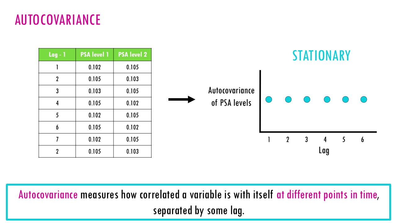
We can then calculate the covariance, or rather, autocovariance, because it’s the same variable: PSA levels in blood, just 1 month apart. If PSA levels are stationary, then the autocovariance should be constant, in other words, it shouldn’t matter that one pair is early in the series and the other is later. Comparing pairs of PSA levels that are 1 month apart should give roughly the same relationship. The “memory” in PSA levels (how much this month’s value depends on last month’s) stays consistent over time, rather than getting stronger or weaker depending on when you measure it.
In summary, for autocovariance to be considered constant (or stationary), that relationship should depend only on the distance between timepoints (the lag), not on when in time you’re looking.
Squidtip
A stationary time series is one whose properties do not depend on the time at which the series is observed.
Example: stationary PSA pattern
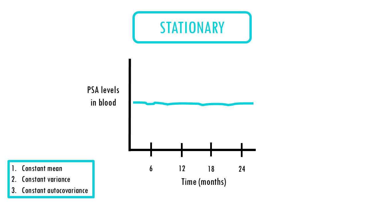
Let’s say a patient’s PSA is being tracked after successful treatment and the cancer is well-controlled, you’d expect something like:
- Constant mean – PSA fluctuates around a stable baseline rather than trending anywhere
- Constant variance – the month-to-month fluctuations (assay noise, minor biological variability) stay similarly sized over time
- No structural drift – a reading from two years ago looks statistically like a reading from last month; nothing about “when” you measured it changes its expected behaviour
This is what a stationary series looks like – noise around a flat baseline, no trend, no widening or narrowing swings.
Squidtip
A stationary time series is one whose properties do not depend on the time at which the series is observed.
Example: non-stationary PSA pattern
As you can imagine, oncology time series, like the levels of PSA in blood, are often non-stationary by design, because the whole point of treatment is to change the trajectory.
A non-stationary PSA pattern, might have
- Trend (drift in the mean) – a steadily rising PSA over successive tests signifies that the mean isn’t constant anymore; it’s climbing.
- Changing variance – as disease becomes more active, PSA readings can become more erratic, not just higher
- Structural break – a treatment event (surgery, radiation, starting/stopping hormone therapy) can create an abrupt shift in the series’ behaviour – the statistical properties before and after the intervention are genuinely different regimes, not just noise
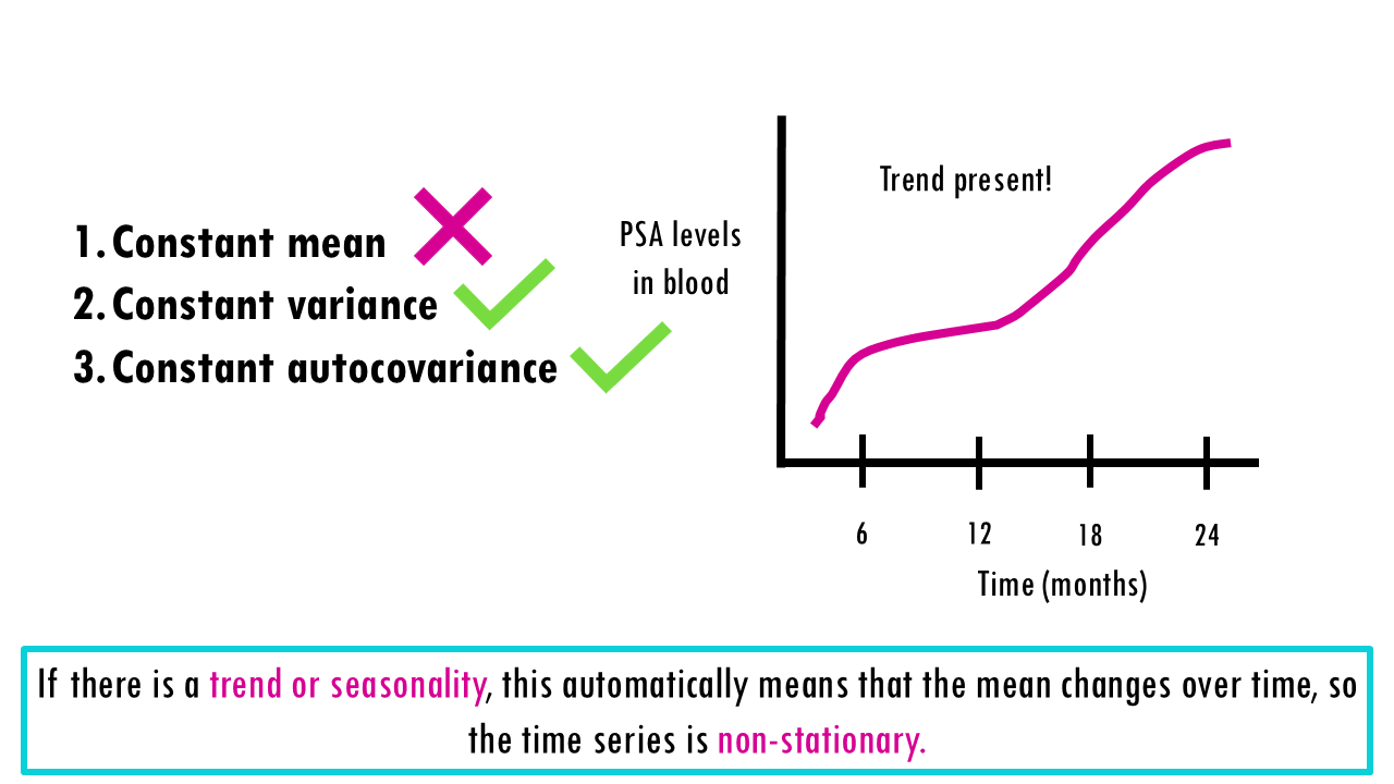
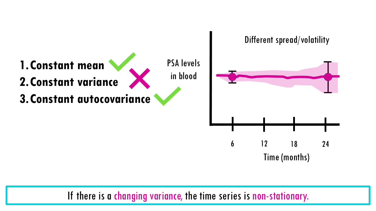
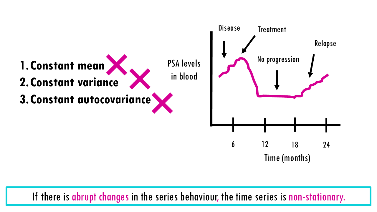
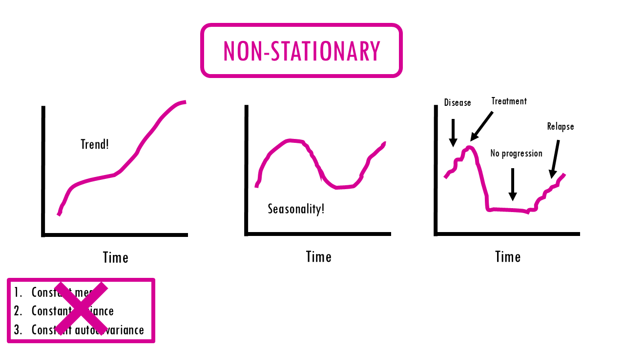
So, essentially, if the mean or variance changes over time, or if there isn’t constant autocovariance, then the series is non-stationary. And this is very important because many classical time series models assume stationarity, so you may not want to use them if you have non-stationary data. There are techniques to transform non-stationary data (like differencing and log or box-cox transforms), but that’s a story for another day!
Squidtip
Many classical time series models assume stationarity!
Irregular sampling
The second challenge that makes medical time series tricky is of course, irregular sampling. Stock prices come in every second. A patient’s blood draws might be 2 weeks apart, then 6 weeks, then 3 months, depending on scheduling and how they’re doing. Real-world clinical time series are messy and unevenly spaced – and the analysis has to account for that, or it will misread noise as signal.
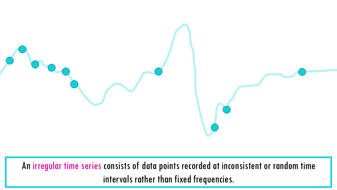
How do we deal with irregular time series?
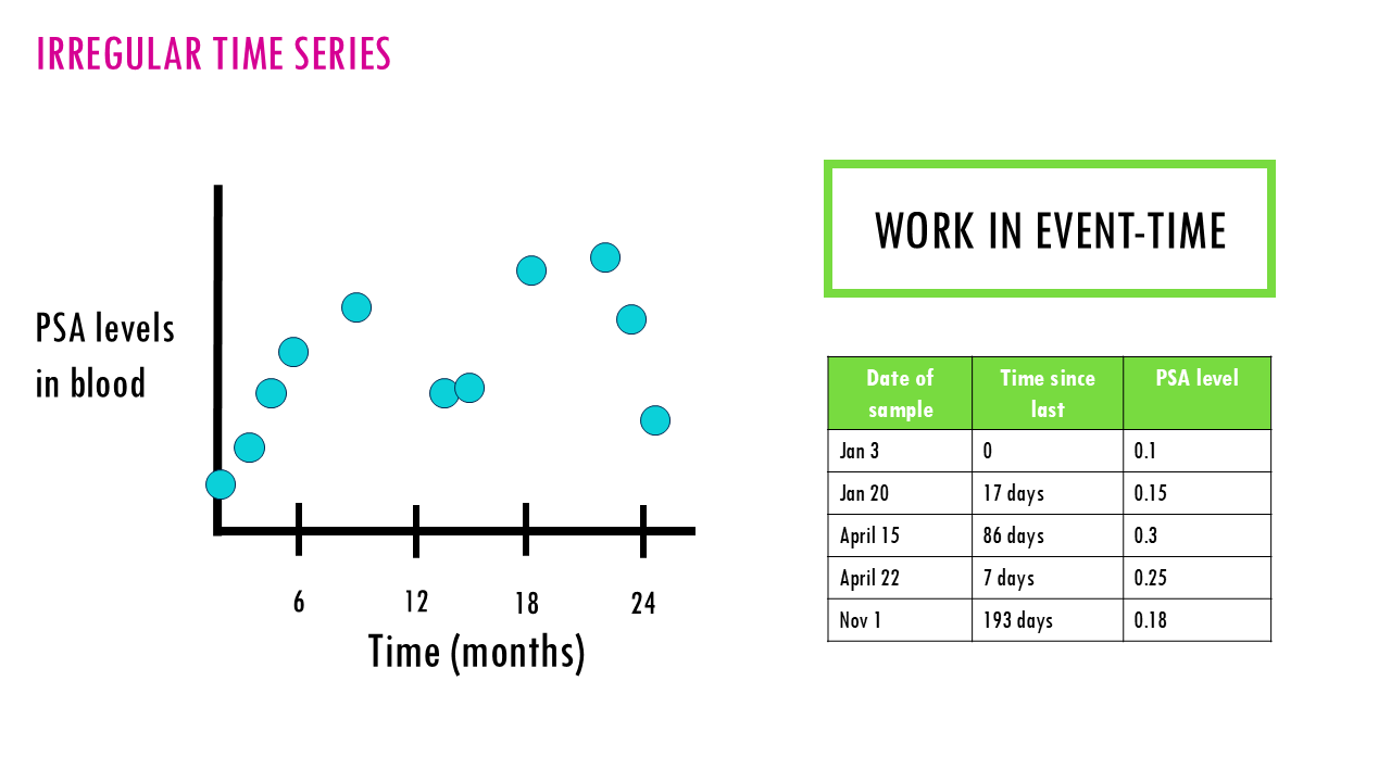
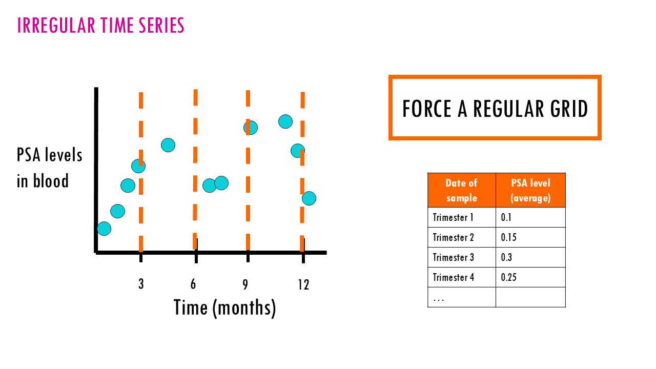
Irregular time series are typically handled by first deciding whether to work in “event time” or force a regular grid.
Event time treats this as: observation 1, observation 2, observation 3… each with its own timestamp and the actual gap to the next one (17 days, then 86 days, then 7 days, then 193 days). You model the data as-is – irregular gaps and all – rather than pretending it arrived on a neat schedule.
Grid time (the alternative) would resample this onto something regular, like monthly values or in this example, trimester values. So you would fill in January to Match with one value, then April to June and so on. Common approaches: resampling/interpolation (linear, spline, or forward-fill, depending on how justified it is to assume values between measurements), aggregation into fixed bins (e.g., averaging all readings within each month).
Another option is to use a model that natively handle irregular spacing – like state-space models/Kalman filters, Gaussian processes, or continuous-time models (e.g., continuous-time ARMA). These models treat time gaps explicitly rather than assuming equal steps. The right choice depends on why the series is irregular: missing-at-random gaps (patient missed an appointment) are handled differently than informative gaps (patient tested more often because something looked concerning, which itself carries signal you don’t want to interpolate away).
Final notes
Squidtastic!
In this blogpost we covered covered time series analysis. Hope it everything was clear! The key takeaway points:
- Time series data is just a sequence of measurements taken at successive points in time.
- Time series can be broken down into trend, seasonality and noise.
- There are stationary and non-stationary time series. A stationary time series is one whose properties do not depend on the time at which the series is observed.
- An irregular time series is a sequence of data points where observations occur at uneven, arbitrary, or unpredictable intervals rather than consistent ones.
Want to know more?
Additional resources
If you would like to know more about ML topics, check out:
- How to Analyse Irregular Time-Series in R (GeeksforGeeks tutorial)
- Time series analysis with tidymodels (tidymodels.org tutorial)
You might be interested in…
Squidtastic!
Wohoo! You made it 'til the end!
Hope you found this post useful. If you have any questions, or if there are any more topics you would like to see here, leave me a comment down below. Your feedback is really appreciated and it helps me create more useful content:)
Otherwise, have a very nice day and... see you in the next one!
Before you go, you might want to check:
Squids don't care much for coffee,
but Laura loves a hot cup in the morning!

If you like my content, you might consider buying me a coffee.
You can also leave a comment or a 'like' in my posts or Youtube channel, knowing that they're helpful really motivates me to keep going:)
Cheers and have a 'squidtastic' day!
