
From a simple train-test split to stratified nested cross-validation!
Imagine studying for a final exam by memorizing the exact answers to a practice test. You might feel like a genius while grading yourself, but if the actual exam asks the same questions in a slightly different way, you’re in trouble. In the world of Machine Learning, we call this “memorization” overfitting, and it is the single biggest hurdle to creating AI that generalizes to the real world. If your model “knows” your dataset too well, it hasn’t actually learned anything—it has just cached the past.
To keep our models honest, we use a series of checkpoints: the Train, Validation, and Test sets. This post breaks down how to architect these splits effectively and explores the power of Cross-Validation—a method that squeezes every bit of insight out of your data without “cheating.”
So if you are ready… let’s dive in!
Keep reading or click on the video to learn about cross-validation for Machine Learning!
Why do we split into train and test sets?
Machine Learning is a big box that includes many different types of algorithms and models, ranging from simple linear regression or a deep neural network. The main purpose of it is to train the model on patterns so that it is able to predict a certain outcome for new data. For example, you might build a model with many clinical and genetic features collected from 1000 patients who responded or not to chemotherapy to then predict whether a new patient is eligible for treatment, or if chemo will most likely not work.
When building an ML model from a dataset, the simplest strategy is to train the model on a subset of your data, let’s say, 80%, and then test it on the other 20% – an 80/20 train-test split.
- The training set (80-90%) allows you to build the model, so it will find patterns based on this subset. The model looks at these examples to learn the relationship between features (input) and targets (output).
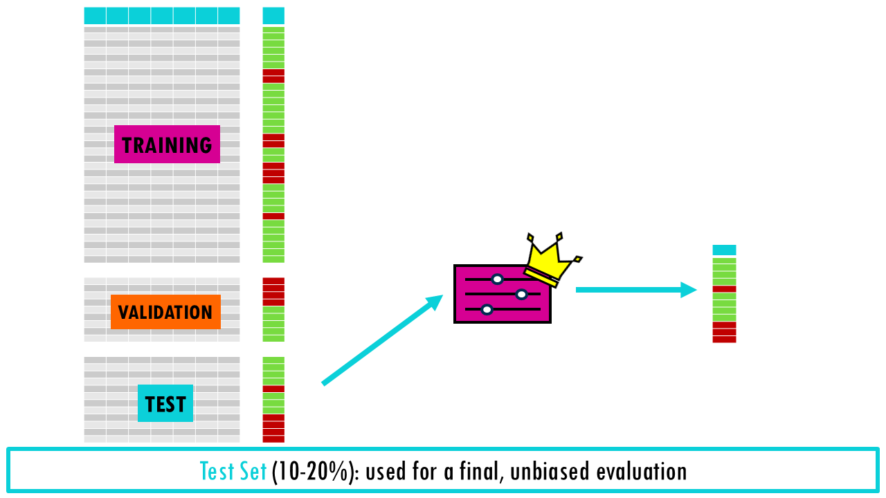
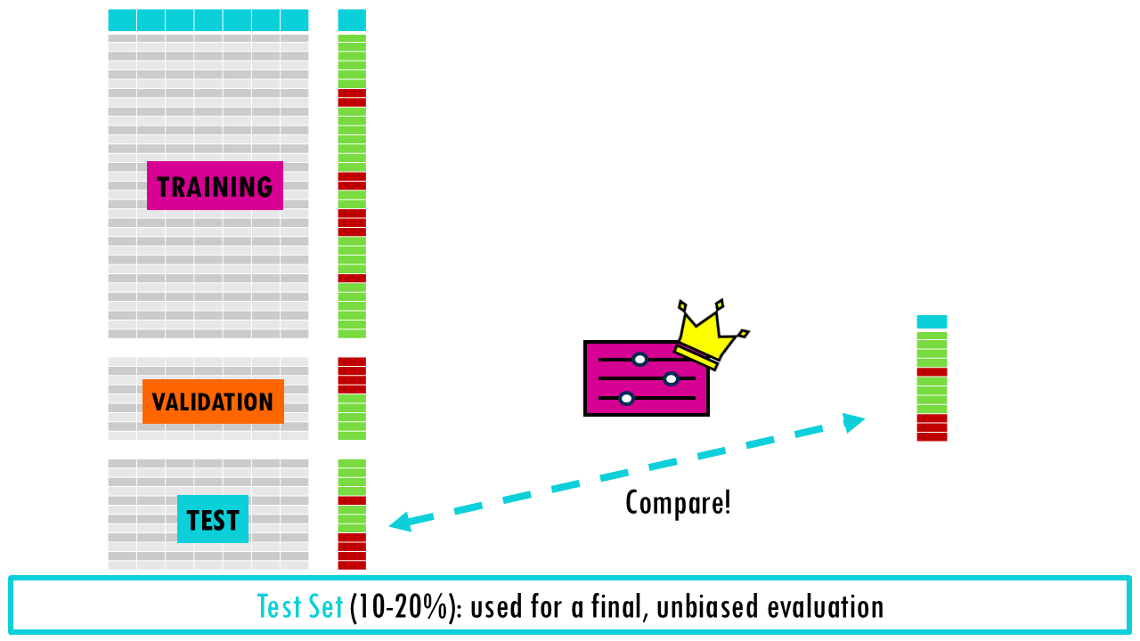
- The test set (10-20%) will allow you to evaluate whether the model is any good at all at predicting outcome. There’s different evaluation metrics which we won’t talk about today, but they all give different measurements of how good the model is at predicting new data.

Squidtip
The percentage splits are only for guidance. If you have a massive dataset (millions of rows), you don’t need 20% for testing. Even 1% might be plenty of samples to prove the model works!
But, why do we split at all?
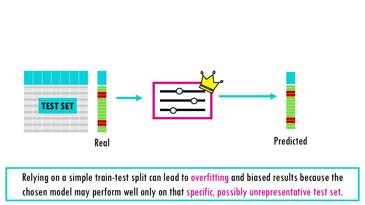
Whether you’re building a simple linear regression or a deep neural network, the “Golden Rule” of machine learning is the same: never test your model on the same data you used to train it. If you do, you aren’t measuring intelligence; you’re measuring memory. If we just train our model with all our data and then evaluate its performance on our data too, it will seem like it’s an amazing model, because the model has already seen these data points and that sample has influenced the model’s pattern-recognition-to-prediction algorithm. This model will be great at predicting your own samples but if you use it to predict new data, it might be completely useless and overfitted to your own dataset: this is what is called overfitting. We should only test the final product on truly “unseen” data to get an unbiased estimate of performance.
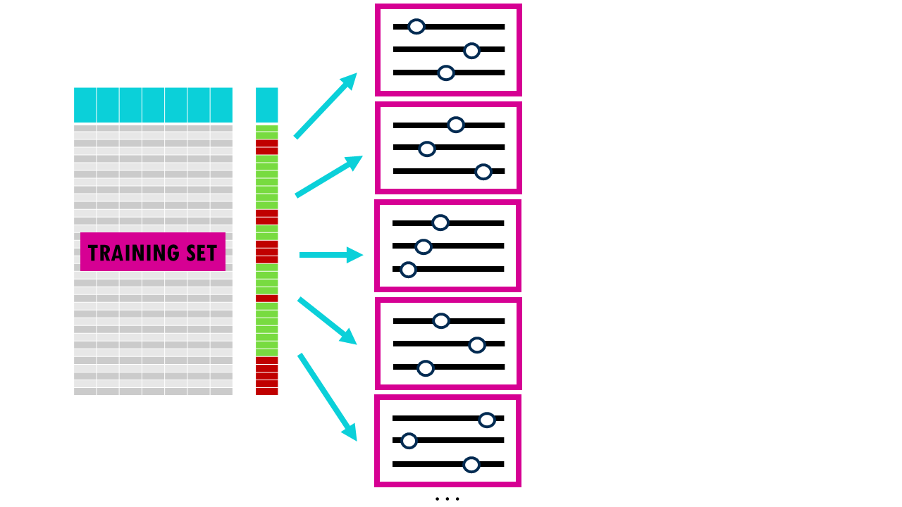
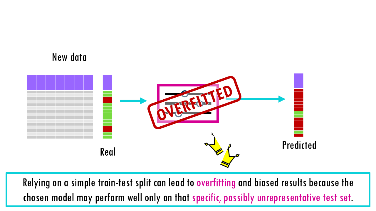
Hold-out method: train, validation and test sets
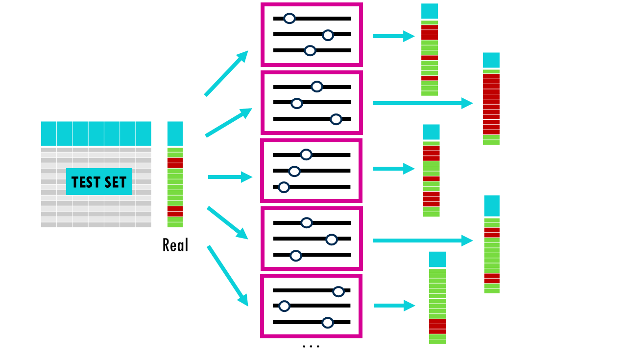
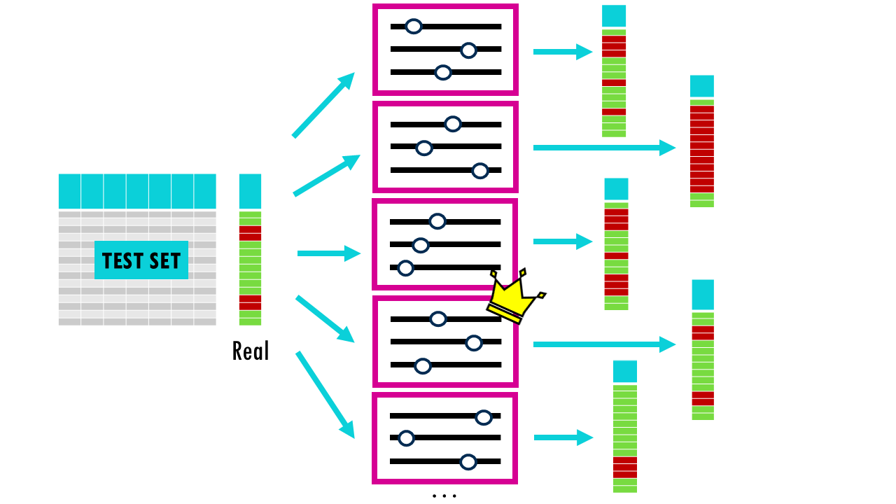
Most models also involve hyperparameters —settings like the depth of a tree or the learning rate—, which we can tune to optimise performance. The idea is that we build different models using different combinations of hyperparameters, evaluate them, and then choose the best one. However, if we just use a simple train-test split, we risk “overfitting” to the test set because we keep tweaking the model until the test score looks good. So we’re essentially choosing the best model according to how it performed in this small subset of data, not necessarily the model that will perform best overall. When we randomly split your data into a training set and a test set just once, you’re relying on luck for how the data gets divided. It’s possible that the test set ends up containing mostly “easy” examples (which any model would get right), making your model look better than it really is. On the other hand, it could contain mostly unusual or difficult cases (outliers), making your model seem worse than it actually is.
Because of this, the test results might not reflect how the model would perform on typical, real-world data – they’re biased by that particular random split.
Squidtip
The model doesn’t “learn” from the validation data directly, but because you make decisions based on it, some information “leaks” into the model. That’s why we need the third test set to get an unbiased performance review of the model.
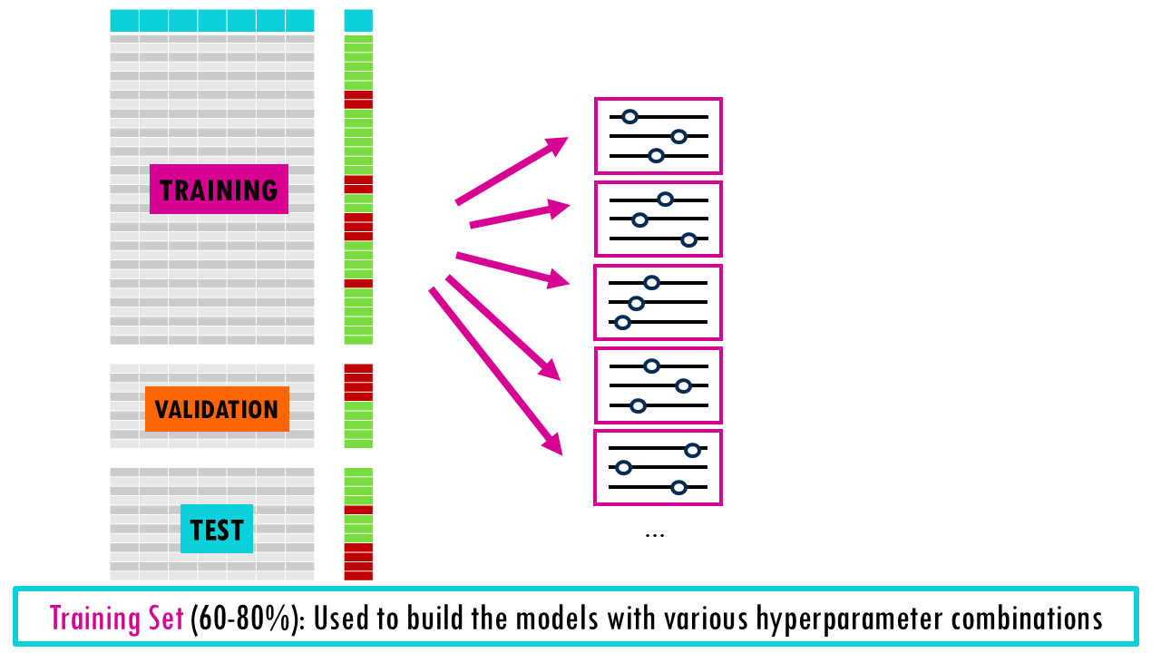
To tune hyperparameters correctly, we split our data into three parts:
- Training Set (60-80%): Used to build the models with various hyperparameter combinations.
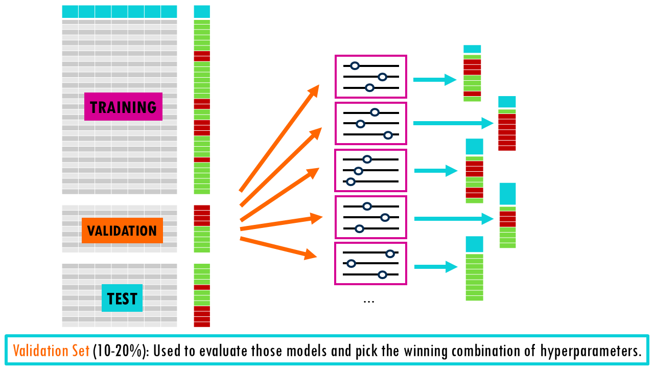
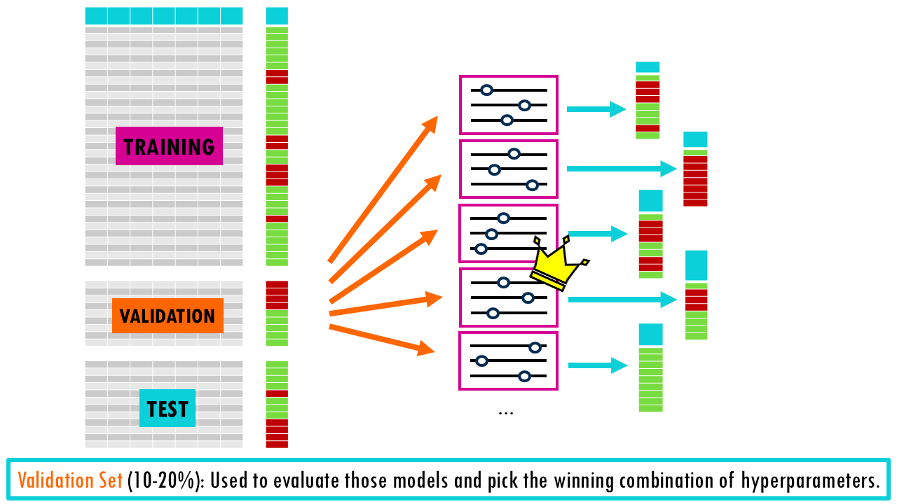
- Validation Set (10-20%): Used as a ‘practice test’ to evaluate those models and pick the winning combination of hyperparameters.
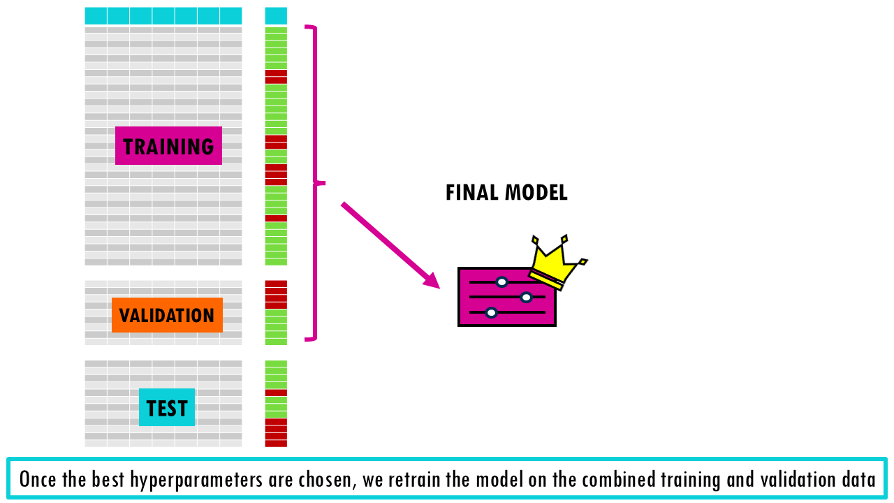
- Test Set (10-20%): Once the best hyperparameters are chosen, we retrain the model on the combined Training and Validation data and use the Test set for a final, unbiased evaluation. It’s very important that test set is only run once to see how your final, chosen model performs. If you use the test set to tweak your model or decide on hyperparameters, it’s no longer a test set—it’s a validation set!
This is called the hold-out method, and while it is fast, it can be “lucky” or “unlucky” depending on how the data is split. If you split the data into 60/20/20, then you are only using 60% of data for training, so the model may miss important patterns in the other half which leads to high bias.
To solve this problem, we can use cross-validation.
Introduction to cross-validation
Cross-validation allows us to check how well a machine learning model performs on unseen data while preventing overfitting and underfitting.
It works by:
- Splitting the training dataset into several parts (called folds)

- Training the model on all but one fold and testing it on the remaining fold (the validation set).


- Averaging the performance across all folds to estimate the model’s generalization performance during model development. For each model with a specific set of hyperparameters, we evaluated the performance on the validation set of each fold.

- The hold-out test set is only used once at the very end and gives the true (unbiased) estimate of generalization performance


Nice! So this is the basic idea behind cross-validation. This method helps reduce problems like overfitting and underfitting and provides a more accurate measure of how well a model will perform on unseen data.
There are different types of cross validation, so we’re going to present some of the most common ones.
K-Fold Cross-Validation
This is the gold standard. The data is split into k equal segments (folds). In each iteration, the model trains on all folds except 1 and validates on the remaining one. This repeats k times so every single data point gets a chance to be in the validation set. Easy!
Let’s say we have 600 samples and we take 100 as the test set. Our training/validation set has 500 samples and we do 10-fold cross validation, meaning we will have 10 folds of 50 samples each. During each iteration, we will train a model on 450 data points, and validate the model on 50 points. Because we are validating the model 10 times, we can get a stable estimate of a model’s accuracy.

Leave-One-Out cross-validation
Leave-One-Out cross validation is basically the same as K-fold cross validation, but each fold is of size 1. This means that only 1 sample point is used as a validation set and the remaining n-1 samples are used in the training set. The model is trained on the entire dataset except for one data point which is used for testing. This process is repeated for each data point in the dataset.
- All data points are used for training, resulting in low bias.
- Testing on a single data point can cause high variance, especially if the point is an outlier.
- It can be very time-consuming for large datasets as it requires one iteration per data point.

Nested cross-validation
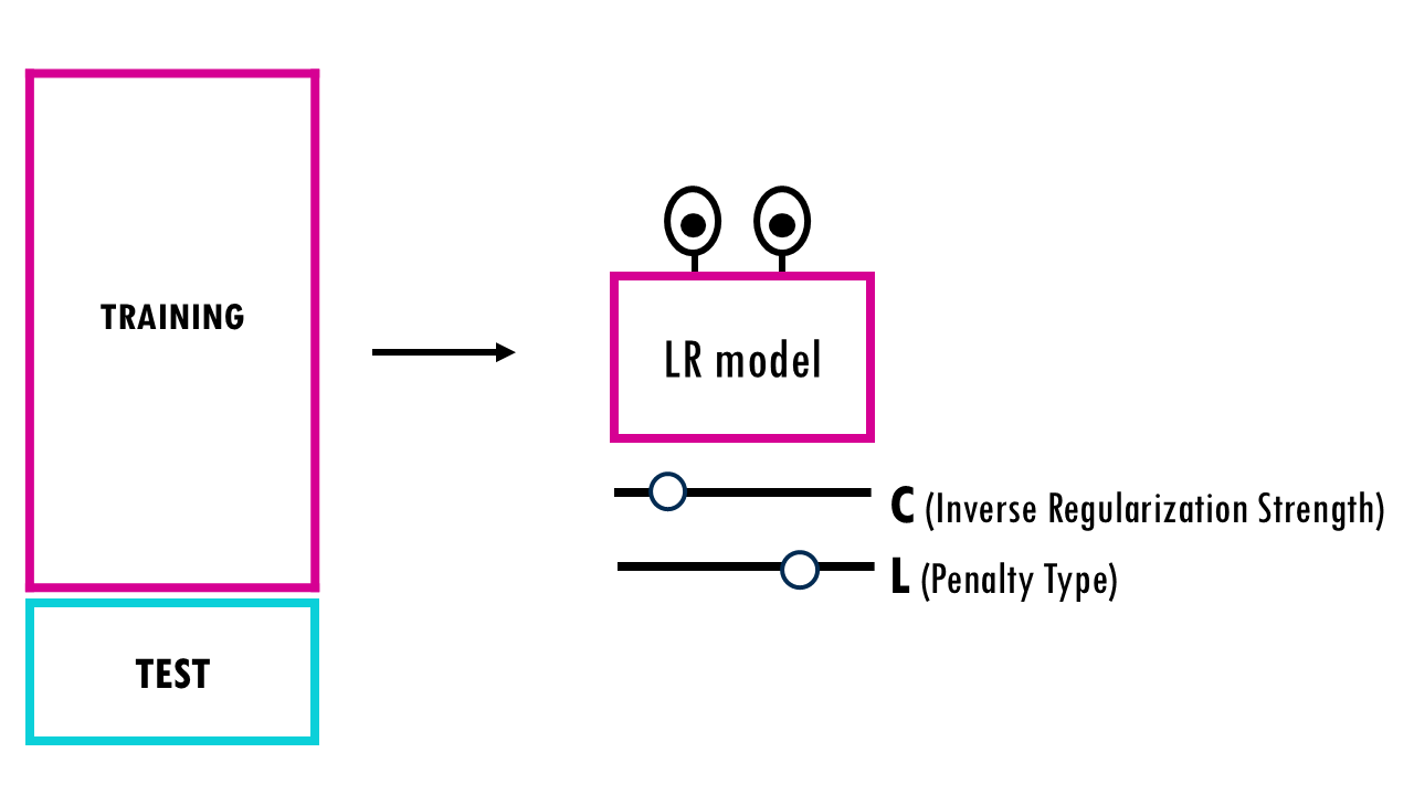
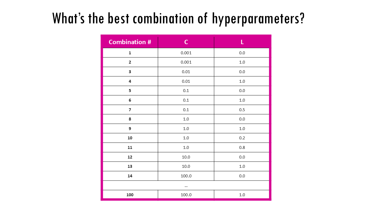
Now, let’s say we want to optimise hyperparameters using cross validation. Just to give a more specific example, we’ll consider a logistic regression model, and we want to optimise hyperparameters C (the Inverse Regularization Strength) or the Penalty Type (L1 vs. L2 or somewhere in the middle) – but this is applicable to all models and their parameters.
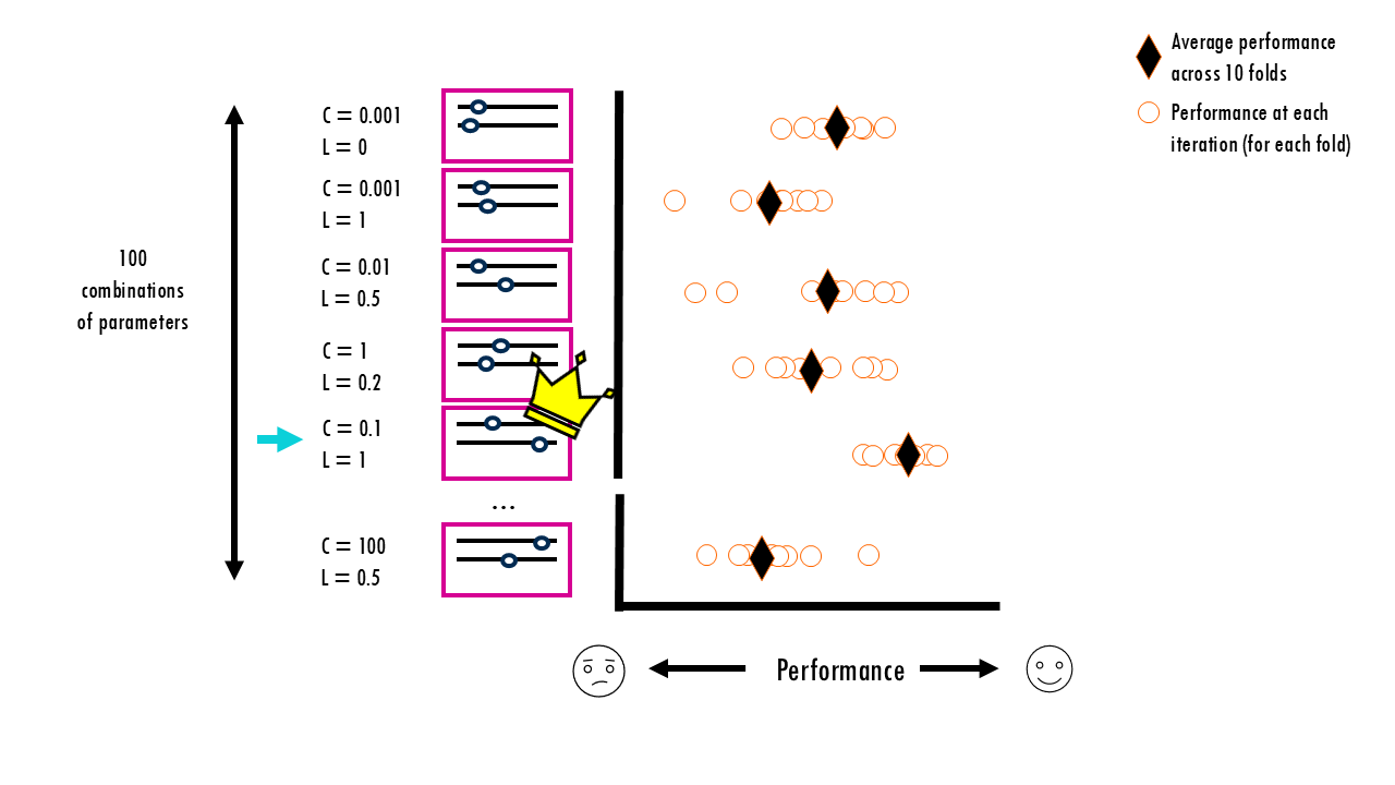
We have 100 different combinations of C and L we want to test out. So we run a 10-fold CV for every single combination, getting an average performance for each of them. Out of our 100 measurements, one specific combination (let’s say C=0.1, L=1) gets the highest average score.
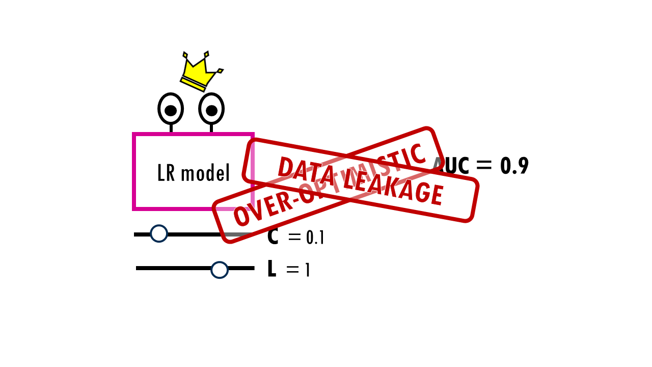
The thing is, even if none of the combinations is truly better, one of them will look best just by luck. The winning combination in our example (C=0.1, L=1) might have won not because it’s the best for all future data, but because its specific settings happened to capture the noise or “quirks” of those specific validation folds perfectly. This is similar to flipping 100 coins 10 times each and picking the one with the most heads—it might just be lucky, not special.
If we report that CV score as our model’s expected performance, we are being over-optimistic. We’ve used the validation results to choose the model so the model is indirectly tuned to those validation folds. This is what is called data leakage – we’ve “leaked” the validation data into your decision-making process. You can see a nice comparison of the performance values between nested versus non-nested CV here.
To get an honest score, you separate model selection from model evaluation.
You need an Inner Loop to pick the best hyperparameters and an Outer Loop to see how those hyperparameters perform on data they’ve never seen.
This is called nested cross validation.
Let’s have a look at how it works with an example.
Squidtip
What is the difference between K fold CV and nested CV? The main difference lies in purpose: K-Fold CV is used to estimate how well a single model performs, while Nested CV is used to both find the best hyperparameters and estimate performance without being biased by that search.
Nested CV explained with an example
In the outer loop, the data (our 500 samples) is split into 10 folds. For each iteration, one fold (50 samples) is put in a “vault.” It is strictly for evaluation and is not looked at during the tuning process.

Now, for each outer loop iteration, the remaining 450 samples are split again (for example, let’s use 5-fold CV). For each combination of hyperparameters we want to test, and in each fold, we train the model on 360 data points, get a performance metric on 90 points, then repeat for each of the folds. That way, we get an average performance across 5 folds per combination. We can then decide on the winner for these specific 450 samples.


Now, we take that winner combination and test it against the 50 samples you put in the vault (the Outer Loop’s validation fold). By the time the model reaches the Outer Loop’s test fold, that data is pure. It wasn’t used to train the model, and—more importantly—it wasn’t used to choose the hyperparameters. The average score across the Outer Folds is a true, unbiased estimate of how your Logistic Regression will perform on totally new points.
We repeat this process for the 10 folds, and we record the performance of each of these “winners” on their respective held-out test folds of the outer loop.

Since we’re using different training rows or samples during hyperparameter selection, for each of the outer loop iterations, we might get something slightly different. For example, we might get something like this:
- Fold 1-4: C=0.1 won.
- Fold 5-8: C=1.0 won.
- Fold 9-10: C=10 won.

If the 10 winners in your outer loop are wildly different (e.g., Fold 1 picks C=0.0001 and Fold 2 picks C=1000), it is actually a huge red flag. It tells you that:
- Your dataset is too small or too noisy.
- Your model is unstable.
- The “best” hyperparameter is just a matter of luck depending on which samples ended up in which fold.
In a stable system, most of the 10 outer folds will pick the same (or very similar) hyperparameters.

So now that we know that our system is stable, we can retrain the model on all 500 samples by performing one final CV search but this time across the entire dataset. Since the Nested CV already proved that our tuning process is reliable and unbiased, we now use all 500 samples to find the absolute best hyperparameters (C and Penalty) one last time.
We retrain it on all 500 samples using standard cross validation, and this is the model we finally test against our original 100-sample true Test Set to see how it will perform in the real world. By keeping those 100 test samples completely separate, you ensure you aren’t just fooling yourself with a model that happened to fit your validation folds perfectly but can’t generalize.

Nice! Remember that the numbers are just examples, there’s different ways of splitting the data and the outer and inner folds don’t necessarily need to be 10-fold and 5-fold – depends on how big your dataset is and other quirks your dataset might have.
Squidtip
Why don’t we just pick the winner out of the 10 folds?
In the example above, if we just “pick” C=0.1 because it won 40% of the time, you are ignoring the data that made the other folds pick something else. Each of those 10 “winners” was chosen using only 90% of your available training data (450 out of 500). To build a model we want it to have seen every single bit of information available.
Nested CV in a nutshell
So, just to recap. Nested CV allows us to simultaneously select hyperparameters (inner loop) and get an unbiased estimate of model performance (outer loop).
We divide our dataset into a training and test set – this is a true test set which will never touched until final evaluation. We’ll only run nested CV on the training set. We split our training set into 10 outer folds. In each outer iteration, 1 of the folds will be the outer validation set, here represented in green, and the rest of the samples will be resplit into 5 folds for the inner CV. This inner CV is used to try every hyperparameter combination by training a model on the gray samples and validating it on the inner validation folds (the orange samples).
The best hyperparameters for each outer fold are chosen based on average inner performance. Now that we have the best hyperparameters for the first outer fold we can retrain it on the whole outer training samples in yellow, and get an unbiased estimate by evaluating it on the outer validation test set (in green). We do this for each of the outer folds, getting 10 unbiased performance estimates, which are then averaged to report the model’s generalisation score.

The key insight is that the outer loop’s validation folds are never used to pick hyperparameters – only the inner loop does that. So the outer loop’s 10 performance scores are genuinely unbiased estimates of how the model generalises. The outer folds evaluated the procedure – they tell us that this pipeline is stable and generalises well. Each outer fold could have chosen slightly different combinations of hyperparameters because they’re based on a different set of samples (the outer training samples in yellow).
To get the final model, we can retrain a model using normal 5-fold CV using all the samples from our training set to choose the final set of optimal hyperparameters and get a final evaluation using the held-out test set.
In conclusion, with nested evaluation we get an unbiased estimate of the model’s performance, we prevent data leakage, get variance and hyperparameter stability insights, and it’s also useful when you have small datasets because you’re maximising the use of all available data.

Stratified K-fold cross-validation
Now imagine you’re trying to build a model for a dataset with class imbalance. Because one of the classes – for example – having a particular disease – is much less frequent, when you shuffle the rows and split the data randomly, you might end up with a test set that contains zero cases for the low frequency class – disease in this case.

Stratification ensures that the proportion of classes in each split matches the original dataset. The data will still be randomly split, but ensuring that the imbalanced feature has the same proportion in both the training and test sets.


This can also be applied to other features too, not only the outcome variable you’re trying to predict. For example, if your data was obtained in 2 different batches (shown in orange and yellow below), you might want to stratify both by the outcome variable and batch. Another common application in biosciences is stratifying by sex, making sure you have similar proportions of females and males in every split.


We’ve seen how to do a stratified train-test split, but of course you can apply stratification to every data split you do. This way we get stratified cross-validation. In stratified cross-validation, for every data split, we ensure the feature of interest has the same proportion in both the training and validation folds.
Stratified K-Fold cross-validation is a variation of K-Fold that ensures each fold has approximately the same percentage of samples of each target class as the original dataset. We can also incorporate stratification into each of our data splits during nested cross validation, giving us stratified nested cross-validation.

Just as a side note, if your class imbalance is really big (usually > 30%) – for example, if you’re building a model to predict survival for a rare disease and only 1 out of 100 cases will have the rare disease – then stratification might not be enough, you might need other machine learning methods that deal with class imbalance such as SMOTE or down/upsampling.
Nice! So we’ve covered train-test splitting for machine learning as well as the main types of cross validation. If you’re dealing with time series data, then you might be interested in time series cross-validation, but that is a story for another day.
Final notes
Squidtastic!
In this blogpost we covered covered train-test splitting for machine learning as well as the main types of cross validation.
Some final, practical tips for effective cross-validation:
- Shuffle Data: Always shuffle your data before splitting, especially for K-Fold cross validation, to ensure each fold is representative of the entire dataset.
- Choose the Right Technique: Select the appropriate cross validation method based on your dataset and problem type (e.g., use time series cross validation for temporal data).
- Evaluate Model Stability: Use cross validation to check the stability of your model. If performance varies significantly across folds, your model might not be stable.
Squidtastic!
Wohoo! You made it 'til the end!
Hope you found this post useful. If you have any questions, or if there are any more topics you would like to see here, leave me a comment down below. Your feedback is really appreciated and it helps me create more useful content:)
Otherwise, have a very nice day and... see you in the next one!
Before you go, you might want to check:
Squids don't care much for coffee,
but Laura loves a hot cup in the morning!

If you like my content, you might consider buying me a coffee.
You can also leave a comment or a 'like' in my posts or Youtube channel, knowing that they're helpful really motivates me to keep going:)
Cheers and have a 'squidtastic' day!
