A step-by-step easy R tutorial for cell type annotation with SingleR
In this easy, step-by-step tutorial you will learn how to to do cell type annotation with the R package SingleR. SingleR is a popular reference-based automatic cell type annotation tool used to predict cell identities from gene expression profiles.
We will go step by step through the workflow, including preparing our input data, running SingleR, interpreting the results and some tips and tricks to get the most out of SingleR.
You will learn how to:
- get normalised counts from your Seurat object
- prepare a reference dataset for SingleR
- interpret SingleR’s cell type predictions (deltas and pruned labels)
- plot the cell types
- add your cell types to your original Seurat object
For this tutorial, I’ll be using RStudio, and you’ll need the packages SingleR, tidyverse. I’ll also use a reference dataset from the package celldex().
If you are more of a video-based learner, you can check out my Youtube video on how to perform cell type annotation with SingleR in R. Otherwise, just keep reading! And remember you can just copy the code by clicking on the top right corner of the code snippets in this post.
Let’s dive in!
Check out my Youtube video to follow this cell type annotation with SingleR tutorial with me!
Click here!
You can also find the script for this tutorial in Biostatsquid’s GitHub page.
Before you start…
In this tutorial, we will learn how to do a cell type annotation of a single-cell dataset using R package SingleR. We will use sample data from the package celldex so if you don’t have a dataset to play around with, you can totally follow this tutorial!
If you are not that familiar with cell type annotation or automatic methods for cell type annnotation, you might want to check publications like this one, or this one. Or you can check my post on cell type annotation for scRNAseq by clicking here.
Let’s talk briefly about SingleR.
When we’re analysing a scRNAseq dataset, at some point, we need to figure out the cell identities of our cells. Are they macrophages? Tcells? Epithelial cells? As you know, a cell identity is based on gene expression: for example, T cells express CD3 (which is a gene that codes for the T cell receptor. Then, different subtypes of T cells express different genes, for example, T helper cells have a higher expression of CD4, whereas cytotoxic T cells express high levels of CD8. Obviously, it does not depend on one gene, but the main idea here is that a cell type is determined by gene expression profile, and the up and downregulation of many sets of genes define a cell type.
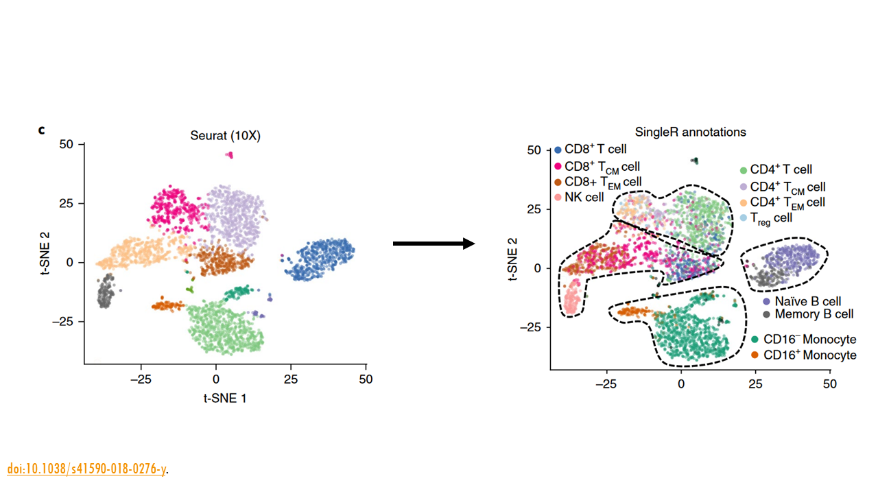
Since a scRNAseq dataset usually has thousands of cells, sometimes tens of thousands, it would be very tedious if we had to look into each of the cells separately, to see what genes they express. That’s where automatic cell type annotation methods come in.
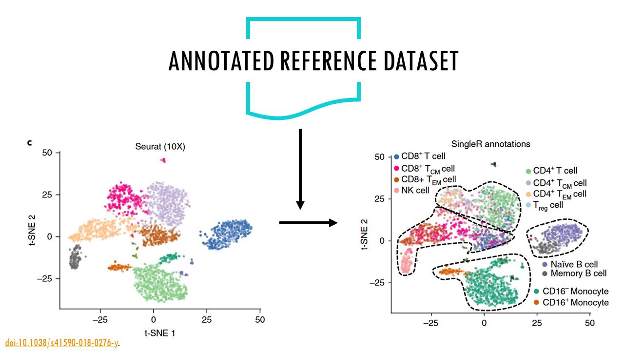
One of the most popular strategies is reference-based annotation. In essence, the algorithm takes a scRNAseq reference dataset that’s already been annotated, and uses the gene expression values from the reference dataset to compare them to your dataset and annotate your own cells. In a way, it transfers the labels from one dataset to the other. This is what SingleR does. Given a reference dataset of samples (single-cell or bulk) with known labels, it assigns those labels to new cells from a test dataset based on similarities in their expression profiles. I won’t go into the method itself, but you can read more about it in the publication.
Great! Ready to start coding?
If you are a beginner in R, don’t be overwhelmed! This tutorial will go step-by-step and I will explain (almost!) every line of code so you know what is happening at each point of the workflow.
For this tutorial you will need R, or Rstudio, and you will need to install the following packages:
BiocManager::install("SingleR")
BiocManager::install("Seurat")
BiocManager::install("tidyverse")
BiocManager::install("celldex")
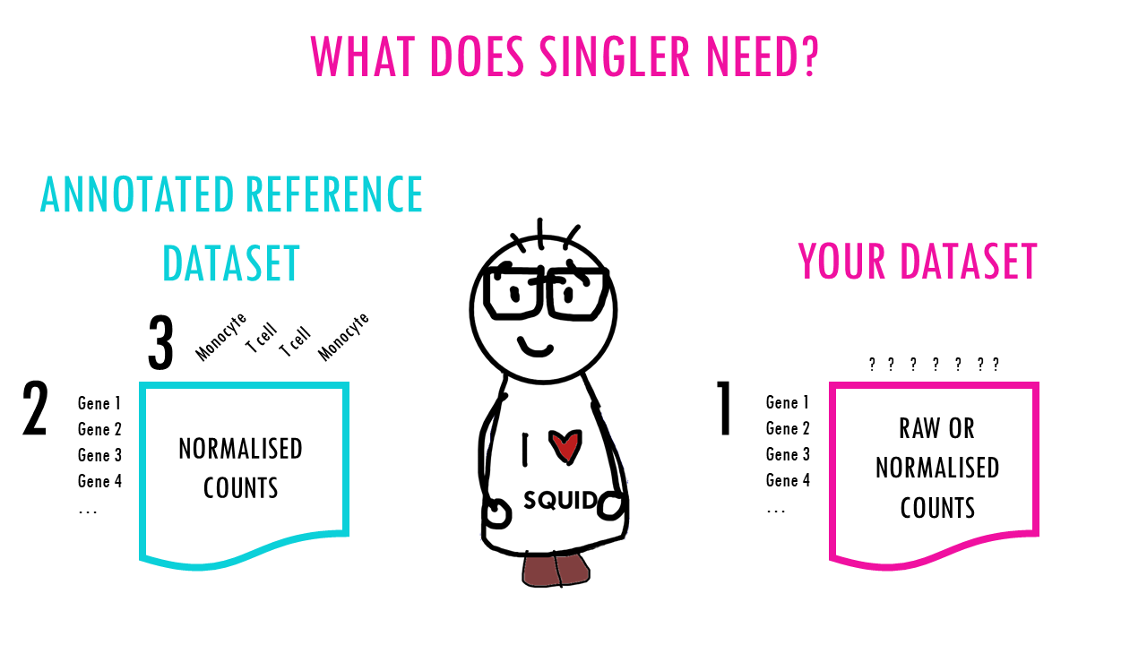
What does SingleR need?
- counts of our dataset (raw or normalised).
- normalised counts of a reference dataset.
- labels of the reference dataset.
Easy! Let’s get started!
Set up your environment
It’s good practice to clear up your environment before you load in any data. This is the general structure I like to keep in all my scripts:
# ---------------------- #
# SingleR_tutorial.R
# ---------------------- #

# Setting up environment ===================================================
# Clean environment
rm(list = ls(all.names = TRUE)) # will clear all objects including hidden objects
gc() # free up memory and report the memory usage
options(max.print = .Machine$integer.max, scipen = 999, stringsAsFactors = F, dplyr.summarise.inform = F) # avoid truncated output in R console and scientific notation

# Set seed
set.seed(42)
We will also need to load the relevant libraries:
# Loading relevant libraries
library(tidyverse) # includes ggplot2, for data visualisation. dplyr, for data manipulation.
library(celldex)
library(SingleR)
library(Seurat)
Preparing inputs
We’ll start by loading the data. I’m going to use a dataset from the scRNAseq package of PBMCs, which are immune cells in the blood. We load it as a SingleCellExperiment (sce) object. SingleR can already take this as input. But since in single cell pipelines it’s more common to work with Seurat objects, we will convert this sce into a Seurat object and extract our counts from there.
# We'll use a PBMC dataset from the R package scRNAseq
sce <- scRNAseq::KotliarovPBMCData(mode = c('rna'))
seu <- CreateSeuratObject(counts = counts(sce), meta.data = as.data.frame(colData(sce)))
rm(sce)
seu <- NormalizeData(object = seu)
# Additional Seurat preprocessing steps -
# This is not necessary for this tutorial but I will use it for visualisation later
seu <- FindVariableFeatures(seu, selection.method = "vst", nfeatures = 2000)
seu <- ScaleData(seu, features = rownames(seu))
seu <- RunPCA(seu, features = VariableFeatures(object = seu))
seu <- FindNeighbors(seu, dims = 1:10)
seu <- FindClusters(seu, resolution = 0.5)
seu <- RunUMAP(seu, dims = 1:10)
1. Get normalised or raw counts
SingleR can use raw or normalised counts from our dataset. I’ll show you how to get both.
In the new Seurat version 5, we extract the raw counts using the function LayerData(), and the raw counts are stored in ‘counts’. Let’s check the raw counts for a few genes and the first 5 samples. To extract the normalised counts, we use the layer ‘data’.
In the code below, I assign raw counts to raw_counts, normalised counts to norm_counts, and then I check the counts for a few genes and the first 5 cells to compare raw and normalised counts.
raw_counts <- LayerData(seu, assay = "RNA", layer = 'counts') #
raw_counts[c('VIM', 'BCL2', 'TP53', 'CD4'),1:5]
norm_counts <- LayerData(seu, assay = "RNA", layer = 'data') #
norm_counts[c('VIM', 'BCL2', 'TP53', 'CD4'),1:5]
> raw_counts <- LayerData(seu, assay = "RNA", layer = 'counts') #
> raw_counts[c('VIM', 'BCL2', 'TP53', 'CD4'),1:5]
4 x 5 sparse Matrix of class "dgCMatrix"
AAACCTGAGAGCCCAA_H1B1ln1 AAACCTGAGGCGTACA_H1B1ln1 AAACCTGCAGGTGGAT_H1B1ln1 AAACCTGCAGTATCTG_H1B1ln1
VIM 2 . 1 2
BCL2 . . 2 .
TP53 . . . .
CD4 . . 1 .
AAACCTGCATCACAAC_H1B1ln1
VIM 4
BCL2 .
TP53 .
CD4 .
> norm_counts <- LayerData(seu, assay = "RNA", layer = 'data') #
> norm_counts[c('VIM', 'BCL2', 'TP53', 'CD4'),1:5]
4 x 5 sparse Matrix of class "dgCMatrix"
AAACCTGAGAGCCCAA_H1B1ln1 AAACCTGAGGCGTACA_H1B1ln1 AAACCTGCAGGTGGAT_H1B1ln1 AAACCTGCAGTATCTG_H1B1ln1
VIM 2.622001 . 1.614255 2.492596
BCL2 . . 2.202576 .
TP53 . . . .
CD4 . . 1.614255 .
AAACCTGCATCACAAC_H1B1ln1
VIM 3.212371
BCL2 .
TP53 .
CD4 . Nice! That’s the first thing SingleR will need. If we check the function with ?SingleR, you can see that the argument test, the dataset we want to annotate, is a numeric matrix were the rows are genes and the columns are cells. Or you can also use SummarizedExperiment object as input if you prefer.
2. Get the reference dataset
Next, let’s find a good reference dataset for our dataset. I’m going to use the HumanPrimaryCellAtlasData() from the R package celldex to annotate our cells. We’ll talk more about the choice of reference datasets at the end of the video in the tips & tricks section. Let’s load the data.
This celldex dataset has label.main, which has rougher or more general cell type labels, and label fine. We’ll go with label.main for this example.
# 2. Get reference dataset
ref <- celldex::HumanPrimaryCellAtlasData()
unique(ref$label.main)
unique(ref$label.fine)Squidtip
The reference dataset you use is crucial, and will have a huge impact on your results.
So… where to get a good reference dataset? More in the tips and tricks section!
Since we have a PBMC dataset, there’s a lot of cell types in the reference dataset, like astrocytes, osteoblasts, hepatocytes.. that are not present in our dataset. This is why I’m going to only keep some blood cell types. However, you need to be careful when removing cell types from your reference, since they may be present in your dataset.
# Subset to include only relevant cell types (CAREFUL!)
ref <- ref[,grepl('DC|B_cell|Neutrophils|T_cells|Monocyte|Erythroblast|
                 Macrophage|NK_cell|Platelets|Myelocyte', ref$label.main)]
unique(ref$label.main)
Squidtip
Since we have a PBMC dataset, there’s a lot of cell types in the reference dataset, like astrocytes, ipS cells, osteoblasts, hepatocytes.. that are not present in our dataset. This is why I’m going to only keep some blood cell types. However, you need to be careful when removing cell types from your reference, since they may be present in your dataset.
Only remove cell types from the reference dataset if you are absolutely, 100% extra sure that the cell type is not present in your dataset.
Run SingleR
Now we’re ready to run SingleR. Excited?
SingleR can take many arguments, but the main ones are:
- test, our normalised/raw counts.
- ref, our reference counts, normalised (you can give it just the matrix of log transformed expression values, but since I have the summarizedexperiment format already, I’m just going to give it this).
- labels, the labels of each of the cells in our reference dataset.
- de.method, the differential expression method it uses to predict the cell types. For single-cell data, the authors recommend the Wilcoxon ranked test.
Let’s run SingleR! It will take more or less time depending on the size of your dataset and your reference.
# 3. Run SingleR
ct_ann <- SingleR(test = norm_counts, # we could also use sce or raw_counts
                  ref = ref,
                  labels = ref$label.main,
                  de.method = 'wilcox')
Nice! Let’s check out the output. As you can see, the function returns a dataframe. We have our cell IDs, the predicted label, and then some statistics on that prediction.
> ct_ann %>% head()

DataFrame with 6 rows and 4 columns
                                                 scores           labels              delta.next    pruned.labels
                                               <matrix>      <character>               <numeric>      <character>
AAACCTGAGAGCCCAA_H1B1ln1 0.327776:0.321938:0.262826:...          NK_cell 0.000000000000000000000          NK_cell
AAACCTGAGGCGTACA_H1B1ln1 0.297983:0.273244:0.231393:... Pre-B_cell_CD34- 0.000000000000000000000 Pre-B_cell_CD34-
AAACCTGCAGGTGGAT_H1B1ln1 0.218938:0.185317:0.199509:...          T_cells 0.566511846755758274874          T_cells
AAACCTGCAGTATCTG_H1B1ln1 0.267314:0.226187:0.235404:... Pre-B_cell_CD34- 0.000000000000000000000 Pre-B_cell_CD34-
AAACCTGCATCACAAC_H1B1ln1 0.258897:0.350308:0.218881:...         Monocyte 0.000000000000000111022         Monocyte
AAACCTGCATGGTCAT_H1B1ln1 0.344614:0.419826:0.266799:...         Monocyte 0.000000000000000000000         Monocyte
What are ‘pruned.labels’ in SingleR output?
What about delta and pruned labels?
Well, by itself, the SingleR algorithm will always assign a label to every cell. But what if the cell’s true label isn’t in the reference dataset? It will still assign it a label. For this and other reasons, SingleR can assign incorrect labels.
The developers tried to mitigate this by removing poor-quality predictions with “low” scores. They basically compute a “delta” value for each cell, which is the gap, or the difference between the score for the assigned label and the median score across all labels. If the delta is small, this indicates that the cell matches all labels with the same confidence, so the assigned label is not very meaningful.
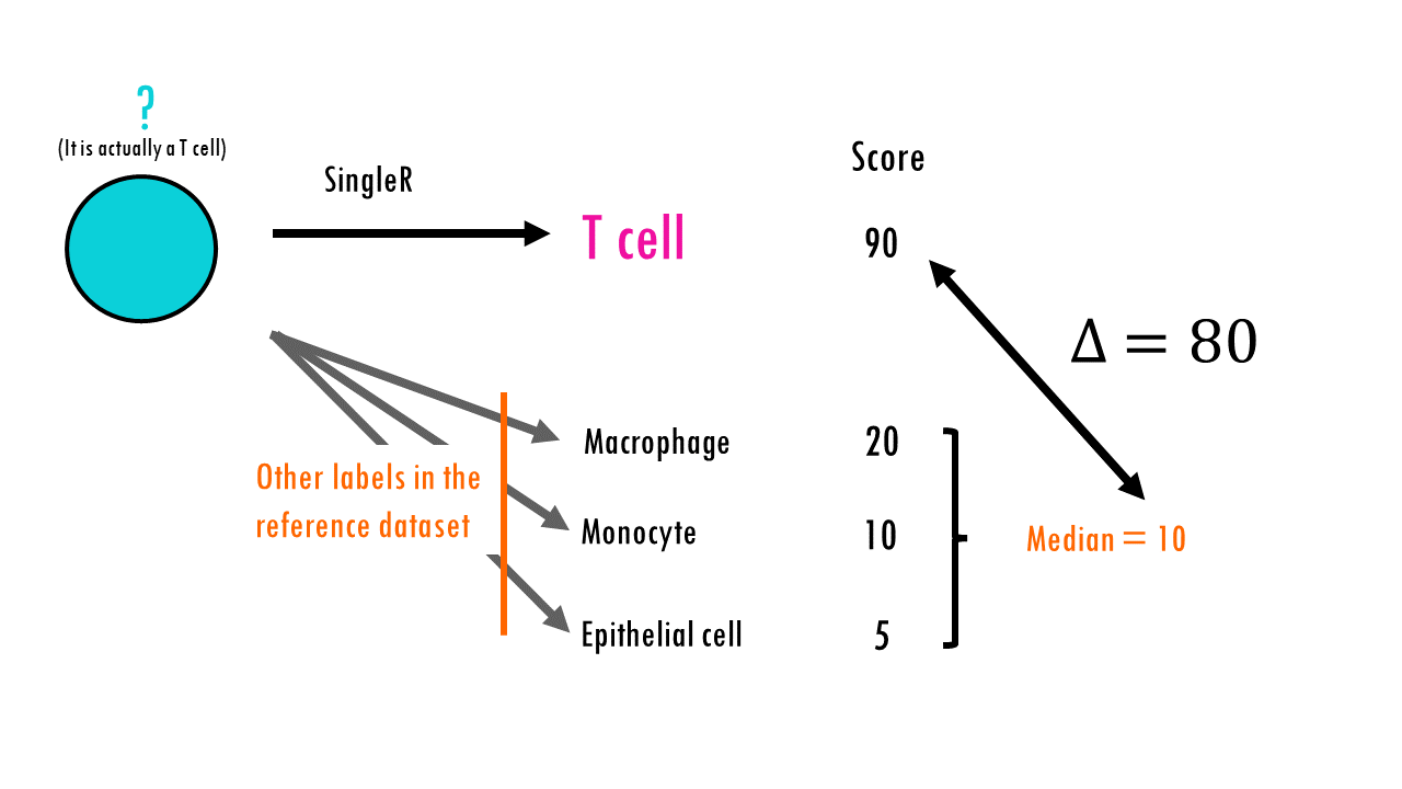
This way, SingleR can discard cells with low delta values caused by (i) ambiguous assignments with closely related reference labels and (ii) incorrect assignments that match poorly to all reference labels – so in the pruned_labels column you will find ‘cleaner’ or more reliable labels.

We can check and compare the pruned labels and the initial labels. As we see the numbers change slightly. And if we check the number of cells without a pruned label, we see that 227 cells were cleaned up and assigned NA because their deltas were too small.
> unique(ct_ann$pruned.labels)

[1] "NK_cell"          "Pre-B_cell_CD34-" "T_cells"          "Monocyte"         "B_cell"
 [6] "Pro-B_cell_CD34+" "Pro-Myelocyte"    "Platelets"        "Neutrophils"      "Myelocyte"
[11] "DC"               "Erythroblast"     NA
> table(ct_ann$pruned.labels)
B_cell               DC     Erythroblast         Monocyte        Myelocyte      Neutrophils
            5580              714              145             8835             1049              736
         NK_cell        Platelets Pre-B_cell_CD34- Pro-B_cell_CD34+    Pro-Myelocyte          T_cells
8764              256            14474              720              313            16841
> table(ct_ann$labels)
B_cell               DC     Erythroblast         Monocyte        Myelocyte      Neutrophils
            5580              714              145             9056             1049              736
         NK_cell        Platelets Pre-B_cell_CD34- Pro-B_cell_CD34+    Pro-Myelocyte          T_cells
8765              256            14475              720              314            16844
> summary(is.na(ct_ann$pruned.labels))
Mode   FALSE    TRUE
logical   58427     227
Inspect the quality of SingleR predictions
We can inspect the quality of the predictions using several functions.
The plotScoreHeatmap function plots a heatmap with the scores. In the y axis we have the different reference labels, which form these rows. Each column is a cell. So we expect cells with a high score for T cells and low for the other clusters to have the final label to be T cells. If the prediction for a certain cell is ambiguous, it will have high scores (yellow) for many of the cell identities. Browse our , with a variety of options to suit every taste and budget, available to buy online.
# Inspect quality of the predictions
plotScoreHeatmap(ct_ann)
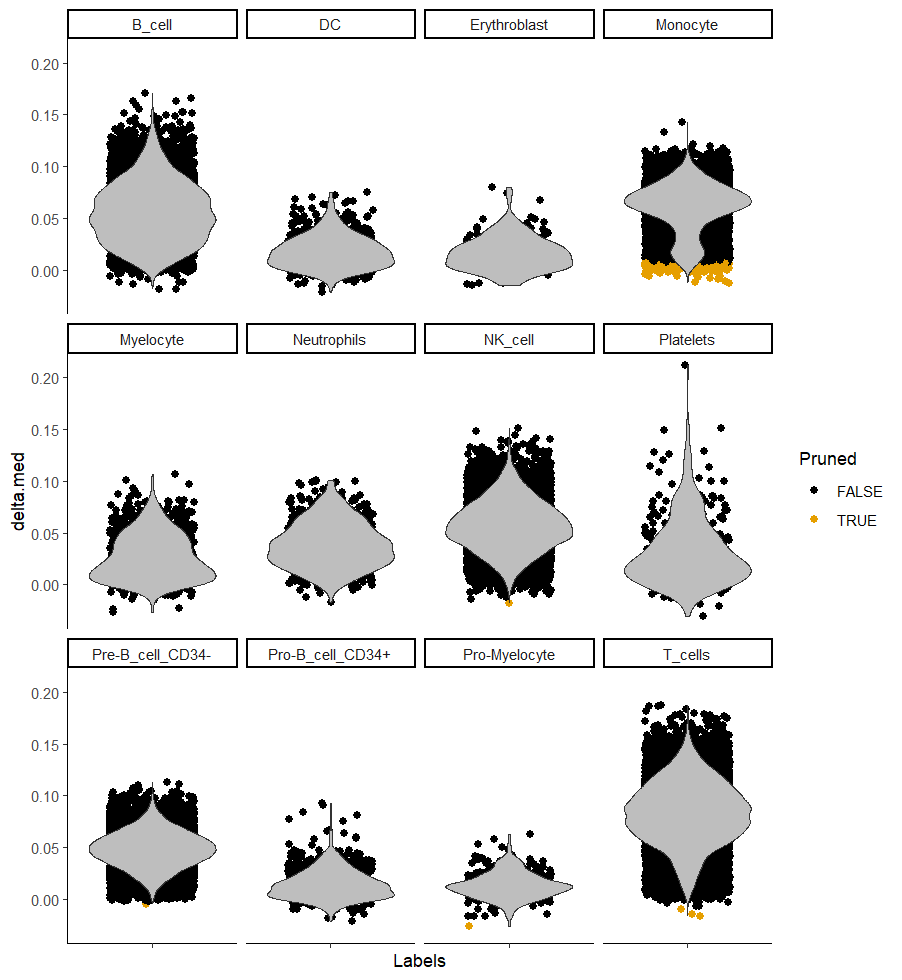
plotDeltaDistribution(ct_ann, ncol = 4, dots.on.top = FALSE)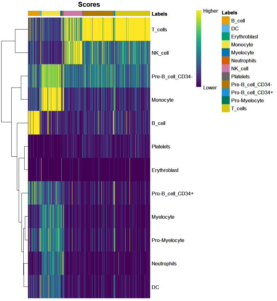
We can also plot the delta distribution. It basically shows the distribution of the gap between the score for the assigned label and the score of the remaining labels) across cells assigned to each reference label. Again, remember that we want high deltas, as they give us more confidence in the assigned label.
Squidtip
You can edit these plots with ggplot functions. For more tips and tricks on how to edit plots in R, check out my other blogpost of visualisation or my Youtube tutorial on top tips to create pretty plots in R.
Add SingleR predictions to Seurat object
Great! So now if you want to add these cell type annotations back to our original Seurat object, you can do it very easily using AddMetadata() from the Seurat object. We just need to make sure that the rownames are the cell IDs that the function will use to match the predictions.
# Add to seurat object
rownames(ct_ann)[1:5] # make sure you have cell IDs
seu <- AddMetaData(seu, ct_ann$pruned.labels, col.name = 'SingleR_HCA')

# Visualise them on the UMAP
seu <- SetIdent(seu, value = "SingleR_HCA")
DimPlot(seu, label = T , repel = T, label.size = 3) + NoLegend()

Cell type annotation tips and tricks
- Use the same gene IDs in your reference and your query dataset. You need to make sure the gene annotation in your reference, is the same as the gene annotation in your dataset! Otherwise it won’t be able to use the genes that don’t match to compare gene expression profiles to predict the cell types.
- Choose a good reference dataset. The reference dataset you use is CRUCIAL. It will define which cell types can potentially be identified in your dataset. So choose your reference dataset carefully. Celldex is an R package that has some nice scRNAseq datasets, but in general it is better to look for publications with as similar methods and tissue of origin as you can. My recommendation is to run SingleR several times with different reference datasets and then find a consensus between all of them – this will give you more reliable cell type annotations.
- Use different annotation methods. Don’t trust a single method to do your cell type annotation! You can use other automatic annotation tools, but also check markers to see if things make sense. If you are interested in more cell type annotation videos, leave me a comment down below!
Squidtip
When doing cell type annotation, it really helps to know what you are looking for, what you are interested in researching. For example, if you are interested in T cells of the liver then you can put more effort into annotating the lymphoid clusters, and you might not care as much about getting very fine labels in your non-immune cell clusters.
Also, take into account that there is no such thing as a cell type. What I mean is that cell type depends on gene expression levels and combinations of genes, and there is a gradient, not defined, discrete profiles. Gene expression also changes temporally and with stresses, so an active CD8+ T cell from the liver is very different from a resting CD8+ T cell from the small intestine. So don’t expect perfect labels, and again, choose your reference wisely!
sessionInfo()
Check my sessionInfo() here in case you have trouble reproducting my steps:
> sessionInfo()
R version 4.3.2 (2023-10-31 ucrt)
Platform: x86_64-w64-mingw32/x64 (64-bit)
Running under: Windows 11 x64 (build 22631)
attached base packages:
[1] stats4    stats     graphics  grDevices datasets  utils     methods   base

other attached packages:
 [1] scRNAseq_2.12.0             SingleCellExperiment_1.24.0 Seurat_5.0.1
 [4] SeuratObject_5.0.1          sp_2.1-2                    SingleR_2.4.1
 [7] celldex_1.8.0               SummarizedExperiment_1.32.0 Biobase_2.62.0
[10] GenomicRanges_1.54.1        GenomeInfoDb_1.38.5         IRanges_2.36.0
[13] S4Vectors_0.40.2            BiocGenerics_0.48.1         MatrixGenerics_1.14.0
[16] matrixStats_1.2.0           lubridate_1.9.3             forcats_1.0.0
[19] stringr_1.5.1               dplyr_1.1.4                 purrr_1.0.2
[22] readr_2.1.5                 tidyr_1.3.1                 tibble_3.2.1
[25] ggplot2_3.4.4               tidyverse_2.0.0

loaded via a namespace (and not attached):
  [1] ProtGenerics_1.34.0           spatstat.sparse_3.0-3
  [3] bitops_1.0-7                  httr_1.4.7
  [5] RColorBrewer_1.1-3            tools_4.3.2
  [7] sctransform_0.4.1             utf8_1.2.4
  [9] R6_2.5.1                      lazyeval_0.2.2
 [11] uwot_0.1.16                   withr_3.0.0
 [13] prettyunits_1.2.0             gridExtra_2.3
 [15] progressr_0.14.0              cli_3.6.2
 [17] spatstat.explore_3.2-5        fastDummies_1.7.3
 [19] labeling_0.4.3                spatstat.data_3.0-4
 [21] ggridges_0.5.6                pbapply_1.7-2
 [23] Rsamtools_2.18.0              parallelly_1.36.0
 [25] limma_3.58.1                  rstudioapi_0.15.0
 [27] RSQLite_2.3.5                 generics_0.1.3
 [29] BiocIO_1.12.0                 ica_1.0-3
 [31] spatstat.random_3.2-2         Matrix_1.6-5
 [33] fansi_1.0.6                   abind_1.4-5
 [35] lifecycle_1.0.4               yaml_2.3.7
 [37] edgeR_4.0.14                  SparseArray_1.2.3
 [39] BiocFileCache_2.10.1          Rtsne_0.17
 [41] grid_4.3.2                    blob_1.2.4
 [43] promises_1.2.1                dqrng_0.3.2
 [45] ExperimentHub_2.10.0          crayon_1.5.2
 [47] miniUI_0.1.1.1                lattice_0.21-9
 [49] beachmat_2.18.0               cowplot_1.1.3
 [51] GenomicFeatures_1.54.1        KEGGREST_1.42.0
 [53] pillar_1.9.0                  metapod_1.10.1
 [55] rjson_0.2.21                  future.apply_1.11.1
 [57] codetools_0.2-19              leiden_0.4.3.1
 [59] glue_1.7.0                    data.table_1.14.10
 [61] vctrs_0.6.5                   png_0.1-8
 [63] spam_2.10-0                   gtable_0.3.4
 [65] cachem_1.0.8                  S4Arrays_1.2.0
 [67] mime_0.12                     survival_3.5-7
 [69] pheatmap_1.0.12               statmod_1.5.0
 [71] bluster_1.12.0                interactiveDisplayBase_1.40.0
 [73] ellipsis_0.3.2                fitdistrplus_1.1-11
 [75] ROCR_1.0-11                   nlme_3.1-163
 [77] bit64_4.0.5                   progress_1.2.3
 [79] filelock_1.0.3                RcppAnnoy_0.0.22
 [81] irlba_2.3.5.1                 KernSmooth_2.23-22
 [83] colorspace_2.1-0              DBI_1.2.1
 [85] tidyselect_1.2.0              bit_4.0.5
 [87] compiler_4.3.2                curl_5.2.0
 [89] BiocNeighbors_1.20.2          xml2_1.3.6
 [91] DelayedArray_0.28.0           plotly_4.10.4
 [93] rtracklayer_1.62.0            scales_1.3.0
 [95] lmtest_0.9-40                 rappdirs_0.3.3
 [97] digest_0.6.34                 goftest_1.2-3
 [99] spatstat.utils_3.0-4          XVector_0.42.0
[101] htmltools_0.5.7               pkgconfig_2.0.3
[103] sparseMatrixStats_1.14.0      dbplyr_2.4.0
[105] fastmap_1.1.1                 ensembldb_2.26.0
[107] rlang_1.1.3                   htmlwidgets_1.6.4
[109] shiny_1.8.0                   DelayedMatrixStats_1.24.0
[111] farver_2.1.1                  zoo_1.8-12
[113] jsonlite_1.8.8                BiocParallel_1.36.0
[115] BiocSingular_1.18.0           RCurl_1.98-1.14
[117] magrittr_2.0.3                scuttle_1.12.0
[119] GenomeInfoDbData_1.2.11       dotCall64_1.1-1
[121] patchwork_1.2.0               munsell_0.5.0
[123] Rcpp_1.0.11                   viridis_0.6.5
[125] reticulate_1.34.0             stringi_1.8.3
[127] zlibbioc_1.48.0               MASS_7.3-60
[129] AnnotationHub_3.10.0          plyr_1.8.9
[131] parallel_4.3.2                listenv_0.9.0
[133] ggrepel_0.9.5                 deldir_2.0-2
[135] Biostrings_2.70.2             splines_4.3.2
[137] tensor_1.5                    hms_1.1.3
[139] locfit_1.5-9.8                igraph_2.0.1.1
[141] spatstat.geom_3.2-8           RcppHNSW_0.5.0
[143] reshape2_1.4.4                biomaRt_2.58.1
[145] ScaledMatrix_1.10.0           BiocVersion_3.18.1
[147] XML_3.99-0.16.1               scran_1.26.2
[149] renv_1.0.3                    BiocManager_1.30.22
[151] tzdb_0.4.0                    httpuv_1.6.14
[153] RANN_2.6.1                    polyclip_1.10-6
[155] future_1.33.1                 scattermore_1.2
[157] rsvd_1.0.5                    xtable_1.8-4
[159] restfulr_0.0.15               AnnotationFilter_1.26.0
[161] RSpectra_0.16-1               later_1.3.2
[163] viridisLite_0.4.2             memoise_2.0.1
[165] AnnotationDbi_1.64.1          GenomicAlignments_1.38.2
[167] cluster_2.1.4                 timechange_0.3.0
[169] globals_0.16.2
And that is the end of this tutorial!
In this SingleR tutorial, I explained how to perform cell type annotation using the R package SingleR. Hope you found it useful and easy to follow!
Before you go, you might want to check:
Squidtastic!
You made it till the end! Hope you found this post useful.
If you have any questions, or if there are any more topics you would like to see here, leave me a comment down below.
Otherwise, have a very nice day and… see you in the next one!
Squids don't care much for coffee,
but Laura loves a hot cup in the morning!

If you like my content, you might consider buying me a coffee.
You can also leave a comment or a 'like' in my posts or Youtube channel, knowing that they're helpful really motivates me to keep going:)
Cheers and have a 'squidtastic' day!


I use cellenic, I have the Normalized Expression Matrix file from each cluster and or all clusters from one treatment. Can you please show me /us how to use that file in this pipeline? I’m very new to R.
I was able to load the celldex package, I loaded my reference database.
but I’m missing the connection btween my file to creating a rda file/object that I can then run through SingleR
Hi! Thanks for your comment. Unfortunately, I’ve never used cellenic, so not sure I can help. You need a matrix of gene expression data, with rownames = gene names and column names = cell IDs. If it helps try running my script to see if you have the same type of data.
Hi, thanks so much for all of your resources!!! Unfortunately when I run SingleR in step 3, I get this error:
> ct_ann = 1.2.0)] useNames = NA is defunct. Instead, specify either useNames = TRUE or useNames = FALSE. See also ?matrixStats::matrixStats.options
I am not able to download older versions of matrixStats – do you have any recommendations? Thanks!
Hi! Hmm, it’s hard to debug with that info only, but from the error message it seems like you specified useNames = NA, you should set it to TRUE or FALSE?