Integration methods in scRNAseq: easily explained!

Single-cell RNA sequencing (scRNA-seq) has revolutionized our understanding of biology by allowing us to measure gene expression in individual cells rather than bulk tissue samples. This technology has generated an explosion of datasets now stored in public repositories like the Gene Expression Omnibus (GEO) and the Human Cell Atlas.

However, there’s a critical challenge: when we want to combine multiple scRNA-seq datasets to answer bigger questions, we encounter batch effects – unwanted technical variations that arise from differences in how the experiments were performed. These batch effects can obscure the real biological signals we’re trying to detect.

We need integration methods that correct for batch effects!

This is part 1 of my series on single-cell RNAseq integration methods. In this blogpost, we’ll cover integration in single-cell RNAseq and get a high level overview of some of the most popular methods to integrate this type of data.

So if you’re ready… let’s dive in!

What are batch effects?

Batch effects are unwanted sources of technical variation that occur due to differences in:

• Sample characteristics: Different donors, tissues, species, or disease conditions
• Experimental protocols: How cells were isolated, handled, and prepared for sequencing
• Sequencing platforms: Different machines or technologies used (e.g., 10X Genomics, Smart-seq2, Drop-seq)

Think of it like photographing the same object with different cameras in different lighting conditions – the object is the same, but the images look different. Data integration methods try to “normalize” these differences so we can see the true underlying biology.

Integration methods for single-cell RNAseq

Many methods and tools to address this challenge in single-cell analyses have been published. But when it’s your turn to integrate datasets, which method do you use?

Let’s get a quick overview of some of the most popular integration methods that are out there. 

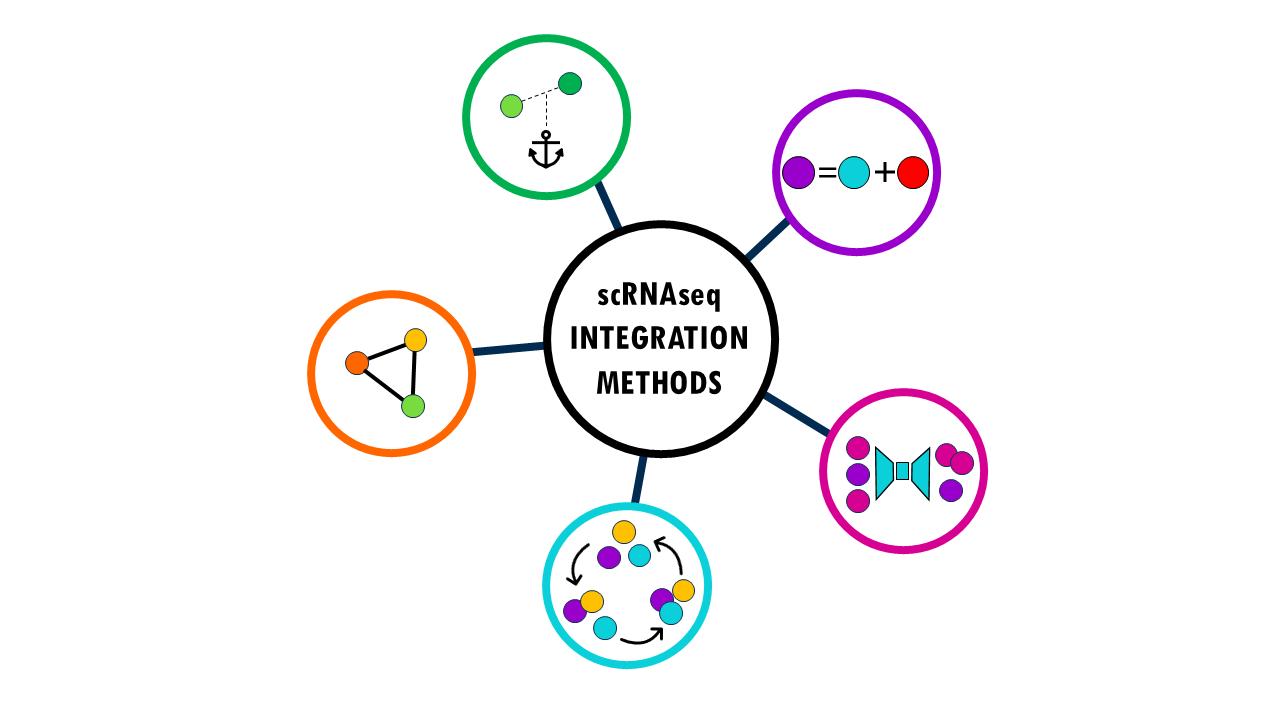
To get a high-level overview, I’ve created 5 different categories in which to classify integration methods. These categories are not “official”, just a way I like to think about all these methods based on the strategy they follow to integrate cells. I’ll briefly present the different integration methods and the strategies they use to integrate data while correcting for batch effects.

Anchor-based methods

The main strategy of these anchor-based methods is to first identify matching or similar cells across batches, and then align data based on these anchors. For example, if you have two brain datasets from two species, it may find certain cell types (dopaminergic neurons, astrocytes…) that are shared cross-species, and it can use those common cell types to, in a way, “overlap” the two datasets. So the key principle here is to match similar cells first, and then integrate.

This is the strategy followed by tools like:

• MNN & FastMNN – Find mutual nearest neighbour pairs between batches; correct batch effects by adjusting cells based on their MNN pairs
• Scanorama – Uses mutual nearest neighbours with “panoramic stitching” to progressively integrate multiple datasets
• Seurat v3 (CCA & RPCA) – Identifies “anchor” cells between datasets using canonical correlation analysis or reciprocal PCA, then integrates based on these anchors.

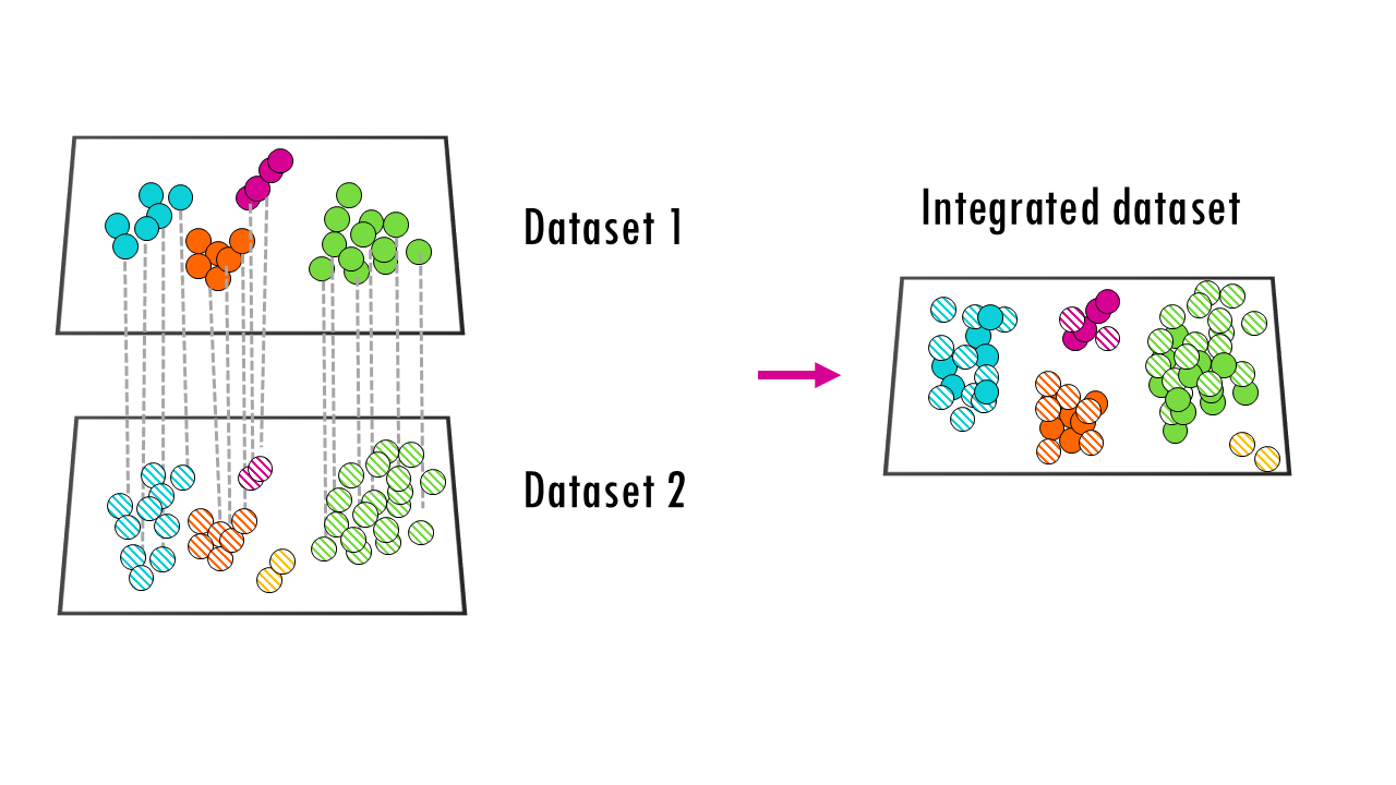
Without going to much into detail, and because Seurat is such a popular package to analyse single-cell data, I’ll briefly mention how CCA and RPCA work. Both use an anchor-based integration strategy with three main steps:

1. Find correspondences: Identify “anchor” cell pairs between datasets
2. Filter anchors: Score and filter anchors to keep high-confidence pairs
3. Integrate: Use anchors to transform datasets into a shared space

The difference lies in how they find the anchors.

Seurat v3 CCA (Canonical Correlation Analysis)

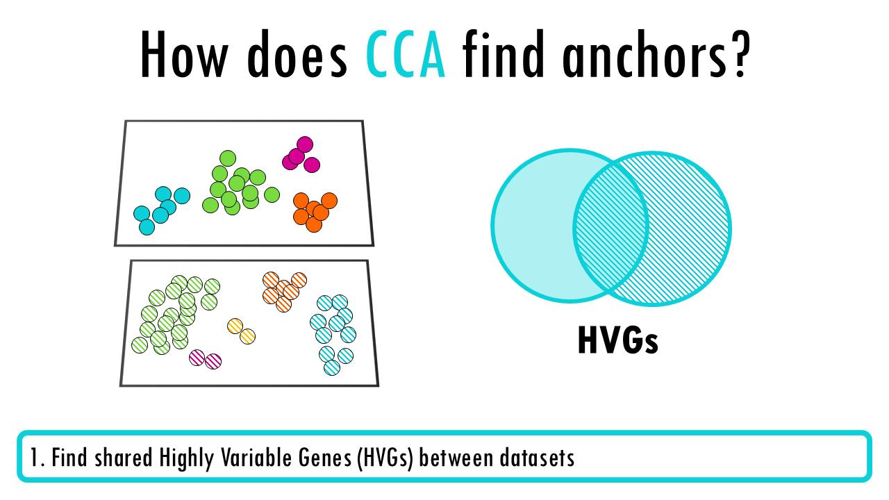
1. Find highly variable genes in each dataset separately
2. Perform CCA on the union of HVGs to find maximally correlated projections between datasets
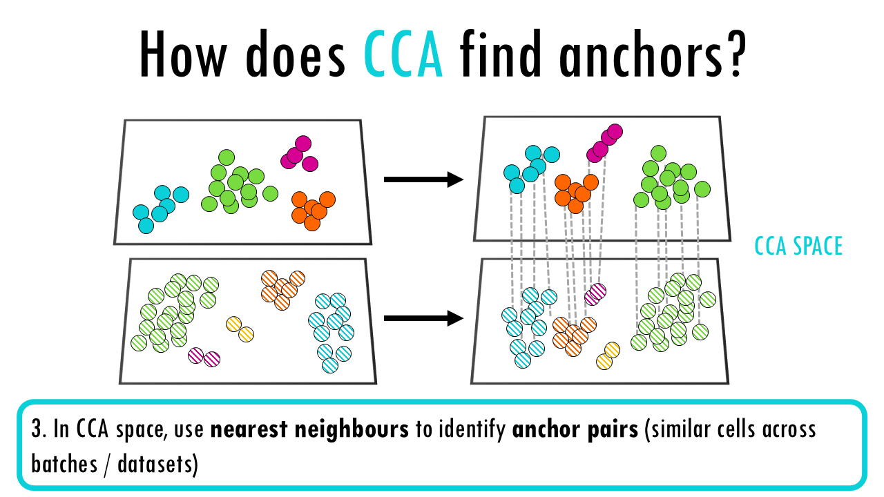
3. In CCA space, use nearest neighbours to identify anchor pairs (similar cells across batches)
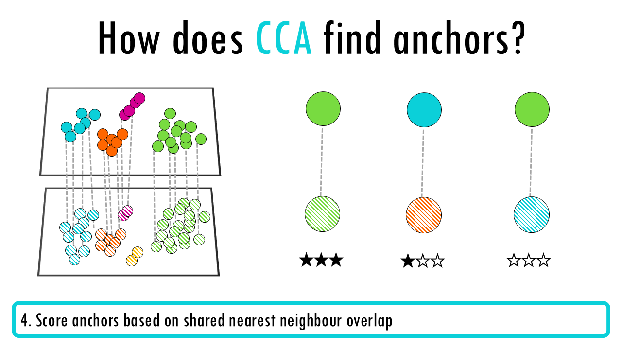
4. Score anchors based on shared nearest neighbour overlap

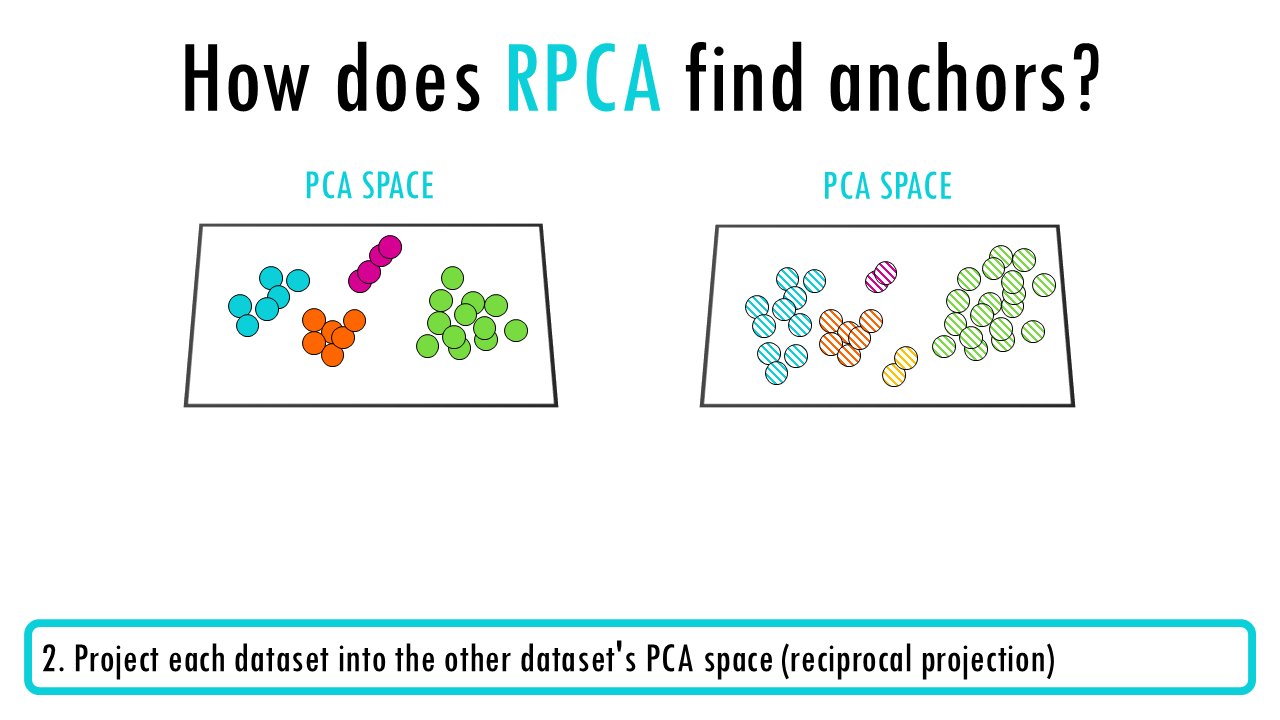
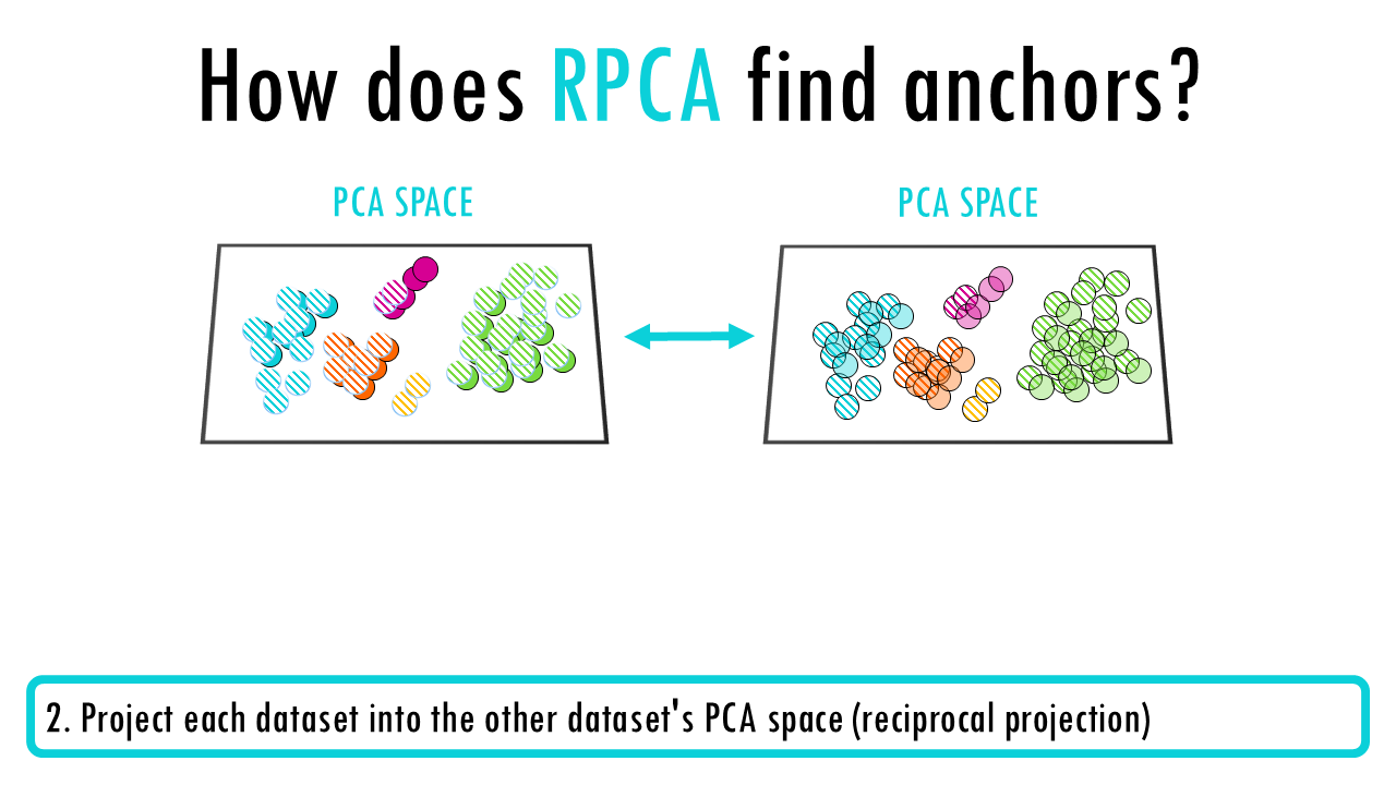
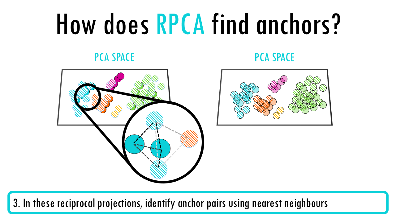
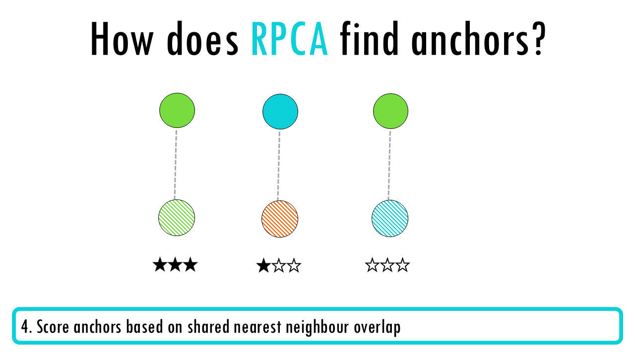
Seurat v3 RPCA (Reciprocal PCA)

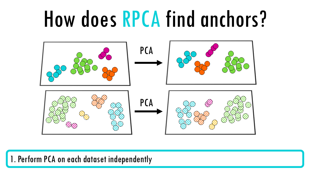
1. Perform PCA on each dataset independently
2. Project each dataset into the other dataset’s PCA space (reciprocal projection)
3. In these reciprocal projections, identify anchor pairs using nearest neighbours
4. Score and filter anchors

Nice! Let’s move on to our next category of single-cell integration methods.

Matrix Factorization Methods

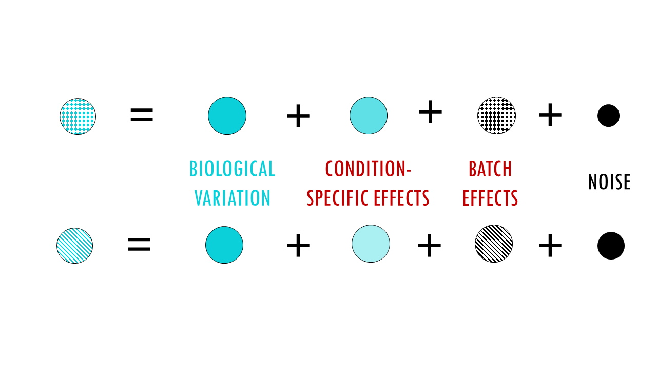
The strategy of matrix Factorization Methods is to decompose data into shared and dataset-specific factors, in other words, they are separating the data into biological variation (to keep) and batch variation (to remove). In essence, they use a mathematical model to separate data into components: overall gene expression, condition-specific effects, batch effects, and noise.

• LIGER – Integrative non-negative matrix factorization that identifies shared factors across datasets and dataset-specific (batch-specific) factors
• ComBat – Uses empirical Bayes to estimate and remove batch-specific parameters from a linear model

Graph-Based Integration

Graph-Based Integration methods construct batch-aware neighbourhood graphs that directly represent integrated cell relationships. The integrated graph is the output; cells are integrated through their connections. Each cell becomes a node in a graph and edges connect cells that are biologically similar.

When constructing the graph, the method makes sure that batch effects don’t cause artificial separation—it chooses neighbors in a batch-aware way. Once this corrected neighborhood graph is built, you don’t get a new expression matrix or corrected coordinates. Instead, the integrated cell relationships are encoded in the edges of the graph itself.

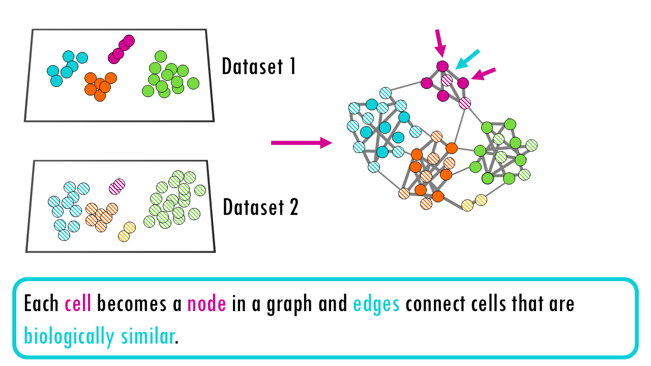
Some integration methods that follow this graph-based strategy are:

• BBKNN – For each cell, samples k nearest neighbours from each batch separately to ensure batch balance (like stratified sampling in the neighbourhood)
• Conos – Builds separate within-batch graphs first, then finds connections between batches by identifying similar cells across datasets and adding inter-batch edges

Iterative Clustering & Correction

I mainly set this category for Harmony, which is a very popular integration method for single-cell RNAseq. Very briefly, these are the steps Harmony follows:

1. Initial setup: Compute PCA on the combined dataset.

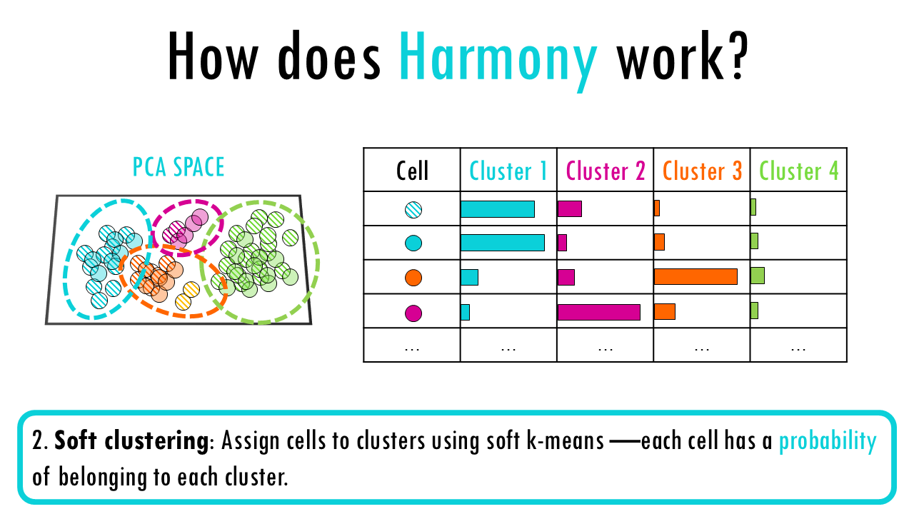
2. Soft clustering: Assign cells to clusters using soft k-means —each cell has a probability of belonging to each cluster. These clusters represent the underlying biological structure the algorithm wants to preserve.

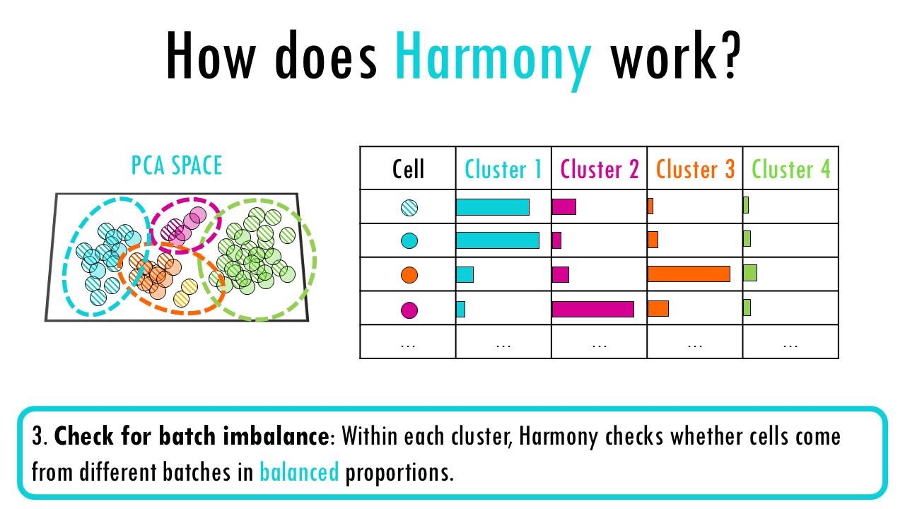
3. Check for batch imbalance: Within each cluster, Harmony checks whether cells come from different batches in balanced proportions.

• • If a cluster is dominated by a single batch → Harmony interprets that as batch bias.
  • If batches are well mixed → no correction is needed.

So essentially, for each cluster, it calculates the expected vs. observed distribution of cells from each batch and then applies a correction to over-represented batches to match the global distribution.

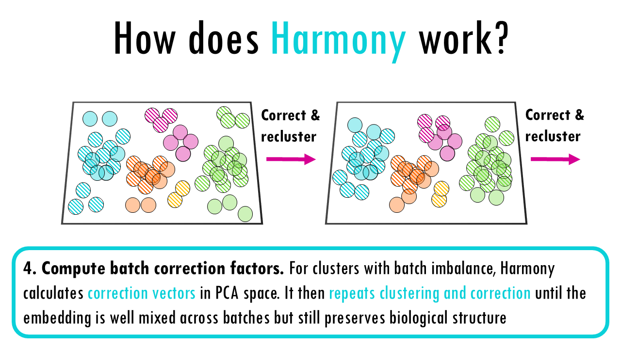
4. Compute batch correction factors: For clusters with batch imbalance, Harmony calculates correction vectors in PCA space. These vectors describe how much to shift cells from each batch so that the clusters become batch-balanced. It then repeats clustering and correction until the embedding is well mixed across batches but still preserves biological structure.

You can read more about Harmony here!

And now, our last category of single-cell RNAseq integration methods… deep generative models!

Deep Generative Models

Deep generative models learn probabilistic latent representations that model both biological variation and batch effects. In plain English, they are models that learn a hidden “blueprint” of each cell that explains both real biology and technical batch differences. They don’t just adjust the data—they learn what variation is biological and what variation is batch noise by modelling the probability of how the data was generated. They try to find out “What would this cell look like if we could see its true biology without the batch effects?”

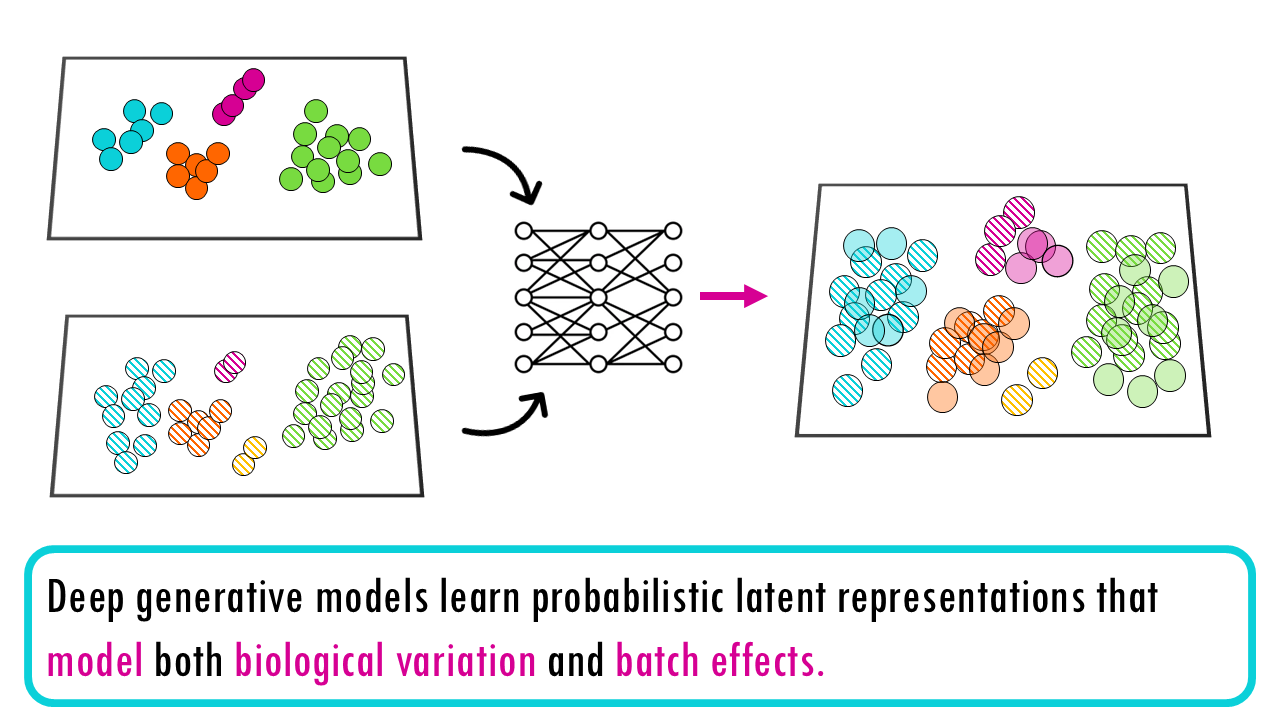
We can distinguish two different types of autoencoders, we’ll explain the differences in just a second. First, let’s get an overview of some of the tools / methods that use this strategy to integrate single-cell data:

• General Autoencoders
  • SAUCIE – Autoencoder with multiple regularization objectives including batch correction
  • DESC – Deep embedding for clustering with batch removal
• Variational Autoencoders 
  • scVI – VAE with explicit probabilistic model for count data and batch effects
  • scANVI – Semi-supervised extension of scVI using cell type labels
  • trVAE – Conditional VAE for modeling perturbations and batch effects
  • scGen – VAE that requires cell type labels to predict responses

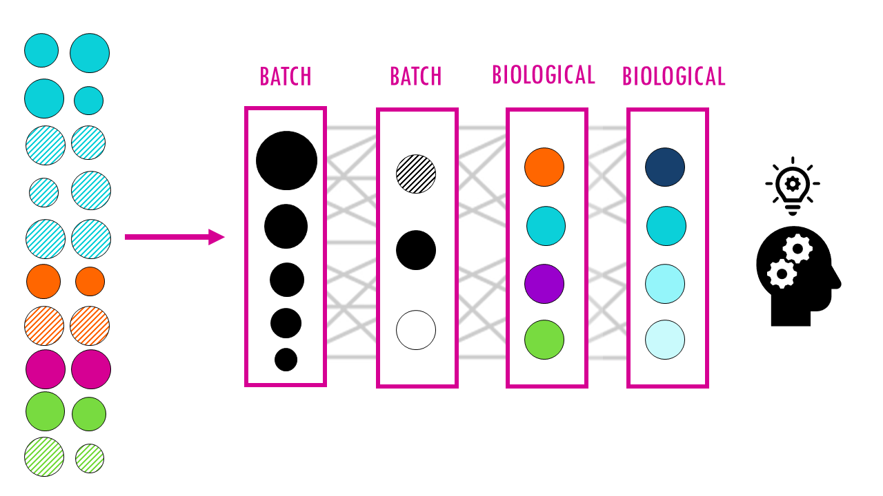
In essence, these methods create a latent space: a compact, hidden representation of each cell. Part of this space captures real biological differences (like cell type) and another part captures batch effects (technical artifacts). The model learns how to separate these sources of variation. Once learned, you can “subtract” the batch part and keep only the biology.

Ok, but… what are (variational) autoencoders?

I’m going to attempt to explain these neural network architectures without any math, but if you’d like a gentle introduction to neural networks, I’d recommend this article. 

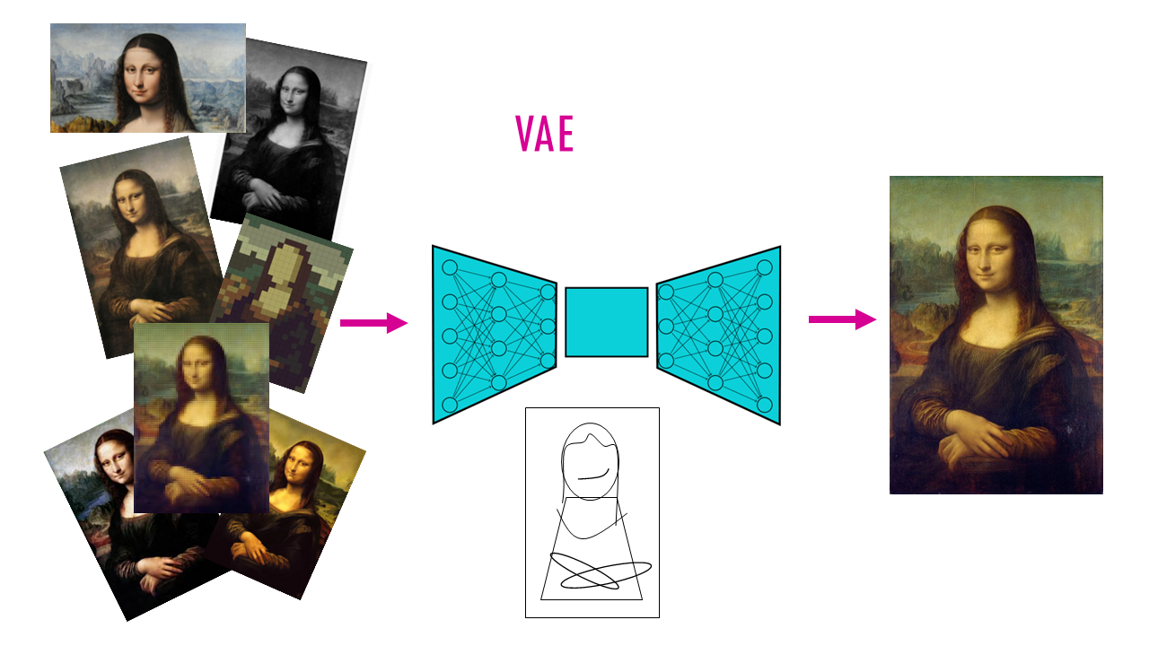
Briefly, a variational autoencoder or VAE has two parts:

• Encoder: Compresses high-dimensional gene expression into low-dimensional latent space
• Decoder: Reconstructs the original data from the latent representation.

If we go back to our original example, our data would be like a bunch of photos taken with different cameras (batches). We want to compare what’s actually in the photos, not the differences between cameras. Variational Autoencoders (VAEs) are like smart compression tools:

• • The Encoder (compressor) will squeeze down out complex data into a simpler form, so instead of thousands of measurements per cell, we keep only a few key numbers that capture the important patterns (like reducing a detailed portrait to “young woman, smiling, outdoors”). So of course, there’s some learning involved where they figure out which patterns are real biology vs. which are just camera artifacts.
  • Then the decoder (decompressor) takes those few key numbers and recreates the full data from them. It’s essentially like regenerating the full photo from the description.

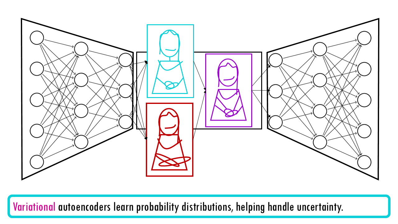
Why “variational”? The “variational” part means it learns probability distributions rather than fixed values, helping handle uncertainty. Instead of saying “this cell is exactly at point X,” it says “this cell is probably around point X, give or take.” This flexibility helps it handle the natural messiness and uncertainty in biological data.

Final notes

In summary, there are many single-cell RNAseq integration methods out there that help you analyse datasets with different unwanted sources of variation. In this blogpost we covered some of the main strategies of current integration methods. Of course there’s many more tools out there than the ones I’ve mentioned, so let me know if you’d like to see a video on any other integration tools, or explain anything with a bit more detail.

So now that it is time to integrate your data, how do you know which method is best? Stay tuned for my next blospost where I’ll go over pros and cons for each method as well as how to choose the best integration method for your dataset!

Want to know more?

Additional resources

If you would like to know more about single-cell integration methods, check out:

• Benchmarking atlas-level data integration in single-cell genomics
• A comparison of integration methods for single-cell RNA sequencing data and ATAC sequencing data
• Benchmarking cross-species single-cell RNA-seq data integration methods: towards a cell type tree of life

You might be interested in…

• UMAPs simply explained
• PCA simply explained
• t-SNE simply explained

Squidtastic!

Wohoo! You made it 'til the end!

Hope you found this post useful. If you have any questions, or if there are any more topics you would like to see here, leave me a comment down below. Your feedback is really appreciated and it helps me create more useful content:)

Otherwise, have a very nice day and... see you in the next one!

Before you go, you might want to check:

Squids don't care much for coffee,

but Laura loves a hot cup in the morning!

If you like my content, you might consider buying me a coffee.

You can also leave a comment or a 'like' in my posts or Youtube channel, knowing that they're helpful really motivates me to keep going:)

Cheers and have a 'squidtastic' day!