Hill numbers and diversity profiles simply explained

Whether you are analyzing a rainforest ecosystem, a human gut microbiome, or a B-cell receptor (BCR) repertoire, the fundamental challenge is the same:

How do we accurately measure the diversity within a single population?

Simply counting the number of unique species or clones rarely provides the full picture. To understand the true structure of these communities, we must account for the relative abundance and distribution of every member. This is where alpha diversity comes in. It provides a standardized mathematical framework that allows researchers across different disciplines to quantify complexity, compare samples, and track how biological communities shift over time.

In our previous blogpost, we covered different diversity metrics, including Shannon and Simpson indices, richness and evenness. These are key concepts used to describe the composition of a population, from ecology to immunology.

However, these indices are not the best way to compare diversity across populations or communities. Let’s find out why Hill numbers are a much better option when describing the diversity across communities.

So if you are ready… let’s dive in!

Why common diversity metrics are not diversities

You might be familiar with diversity metrics like the Shannon, Simpson, Gini , Chao1 indices. (If you are not, check out this other blogpost first!).

However, they are often misinterpreted in diversity studies. 

You see, these indices are not diversities. They are entropies.

This idea was introduced by Lou Jost in 2006, and it revolutionised how we think about diversity. He argued that most standard indices (like Shannon or Simpson) are entropies, not diversities, and that this distinction is crucial for making accurate biological comparisons. 

Ok, so what is the difference between entropy and diversity?

Entropy measures uncertainty or concentration in a probability distribution. The metrics we mentioned (Shannon, Gini-Simpson…) measure the uncertainty in predicting the identity of one or two individuals drawn at random from a community.

The problem is that these measures are non-linear. For example, if you have a forest and you double the number of equally common species, the Shannon entropy does not double. This makes them counterintuitive for comparing different sites.

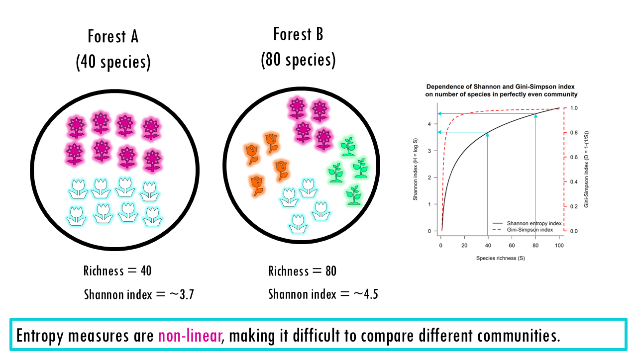
To make them linear, or to speak “biologically”, we must convert these entropies into effective numbers of species (also known as Hill Numbers).

To give you a simple metaphor. Raw indices (Shannon, Simpson) are like measuring temperature in some abstract unit. Hill numbers convert them into “degrees” everyone understands — effective species counts. You still get the same information, but in a form that’s interpretable, comparable, and mathematically well-behaved.

So how do we “transform” entropies into effective number of species?

Hill numbers

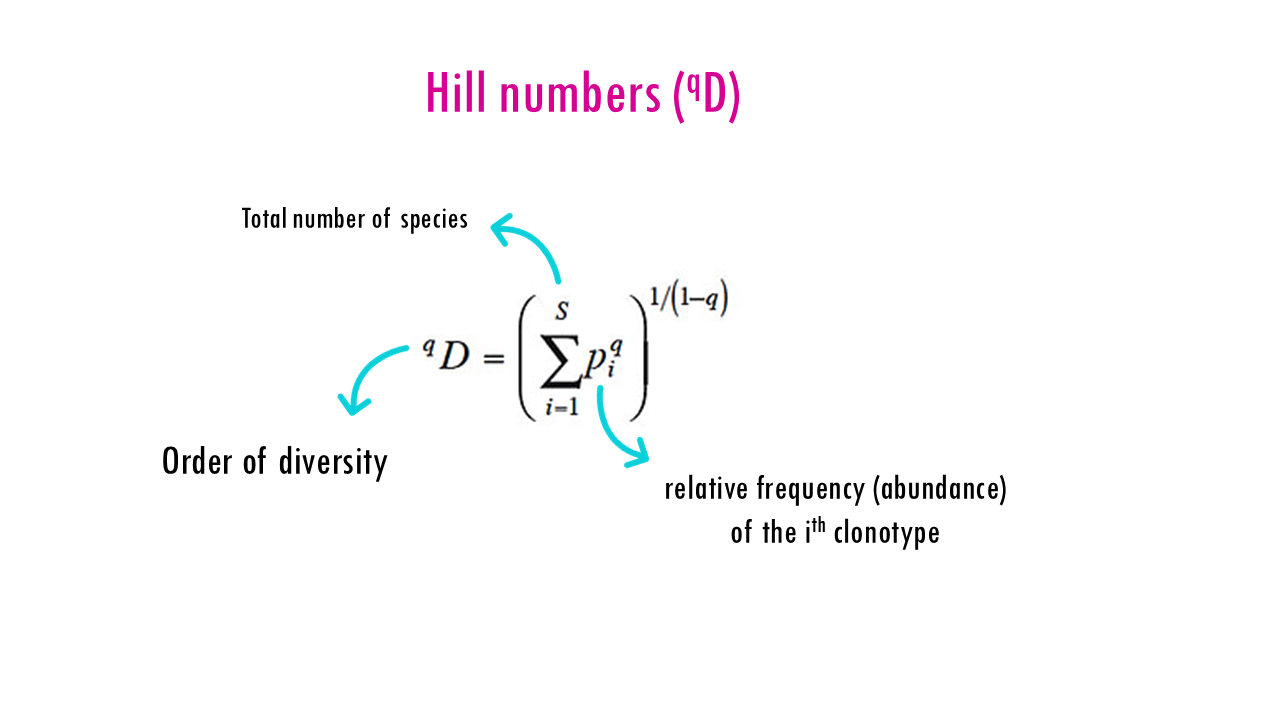
Note on q = 1: The formula is undefined at exactly 1, but as q approaches 1, it becomes the exponential of the Shannon entropy.

The order “q” defines how we measure diversity

One of the key points of Hill’s equation is that Hill numbers depend on the parameter q, which is the “order”. So you can calculate Hill numbers for different orders.

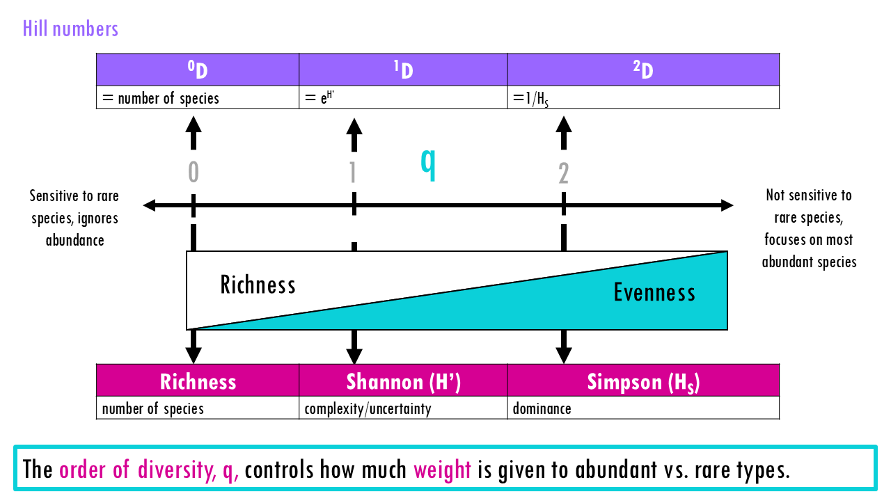
As q increases, the index becomes less sensitive to rare species (for example, in BCR sequencing, they would be called singletons) and more sensitive to dominant species (or highly expanded clonotypes). So q controls how much weight is given to abundant vs. rare types.

Does this ring a bell?

Hill numbers at specific values of q relate to the diversity indices we’ve already talked about.

• If q = 0, we get richness, or the total number of unique clones.
• If q = 1, we get the exponential of Shannon entropy.
• If q = 2, we get the inverse Simpson metric.

How to interpret Hill numbers

Let’s explain now why Hill numbers make interpretation and comparison between communities much easier.

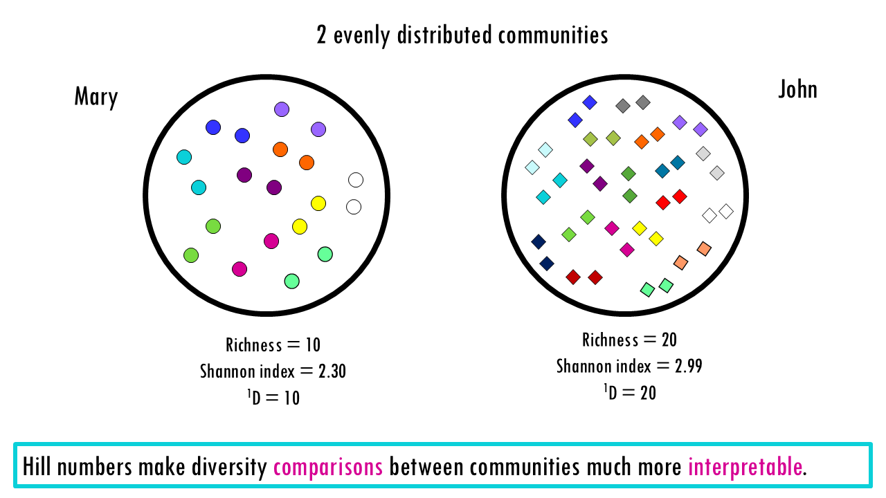
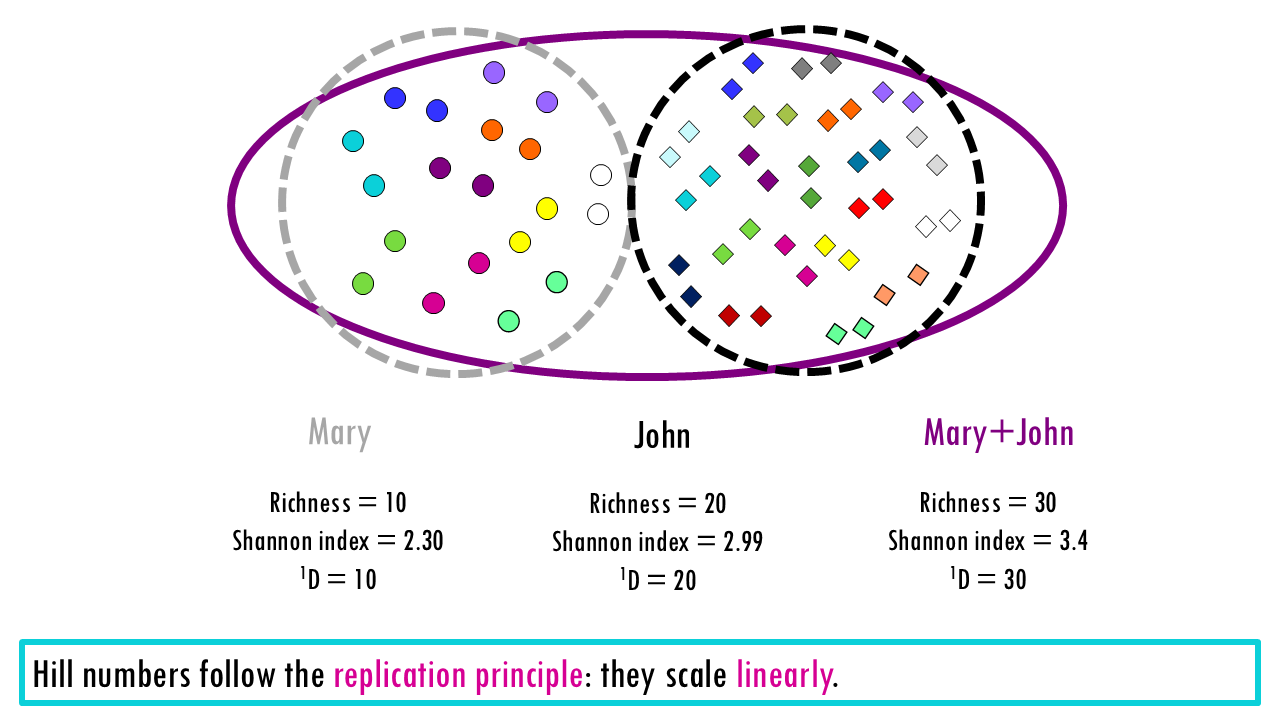
Let’s start with a simple example of 2 evenly distributed communities, in this case, the BCR repertoire of two patients, one has 10 unique BCRs and one has 20 unique BCRs. The richness is therefore 10 and 20. Now let’s look at the Shannon index, which gives us a balanced view between the more rare and more expanded clonotypes (although in this case all clonotypes are equally distributed). As you can see, intuitively we would say that patient B is twice as diverse. However, looking at the Shannon index, The value goes from 2.30 to 2.99. Looking at these values, it is not obvious that diversity has doubled.

If we now calculate the corresponding Hill numbers, at q = 1, the value goes from 10 to 20. The effective number of species of John is double than that of Mary, which makes sense, as it has double the amount of even clonotypes. This is an example of how Hill numbers make comparisons much more immediate and logical. The Hill numbers in this case are saying, that if we measure diversity “according to Shannon”, Mary has “effectively 10 evenly-distributed clonotypes” and John has “effectively 20 evenly-distributed clonotypes”. (Note that in this case the actual richness and Hill numbers at q = 1 match because we do have evenly distributed communities). 

Another advantage of Hill numbers is that they follow the replication principle. If we combine both communities or the BCR repertoire of these two patients, the Shannon index doesn’t scale linearly, so it makes comparing communities much less intuitive. Hill numbers add up – the total diversity of both patients is 30 (note that they don’t have any overlapping clonotypes!). 

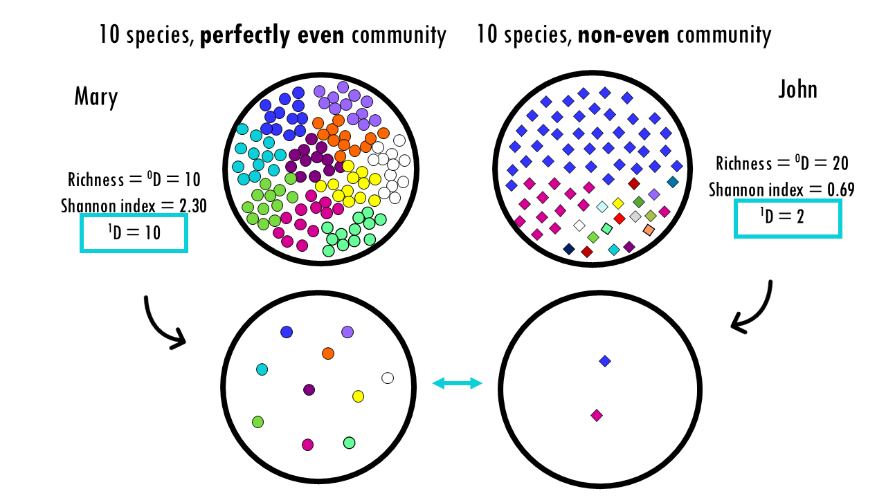
Ok, this was with a perfectly even community, but most real-life examples are communities that are not even, for example, when a few clones dominate. What would happen in a non-even community? 

Let’s imagine both Mary and John have 100 clonotypes, or BCRs, but in the case of John, 1 or 2 clonotypes dominate. Again, the diversity indices don’t really allow us to easily compare both communities. But if we convert these to Hill numbers, this tells us the effective number of species: 10 for Mary and 2 for John.

So what does a D of 10 or 2 mean in this case? This is telling us that if we measure diversity in Shannon’s terms – which, if you remember is a balance between expanded and non-expanded clonotypes – then Mary’s diversity is equal to having 10 evenly-distributed clonotypes (which it actually has), and John’s diversity is equal to having 2 evenly-distributed clonotypes.

In other words, John’s uneven clonotype repertoire is as diverse as an even community of 2 species.

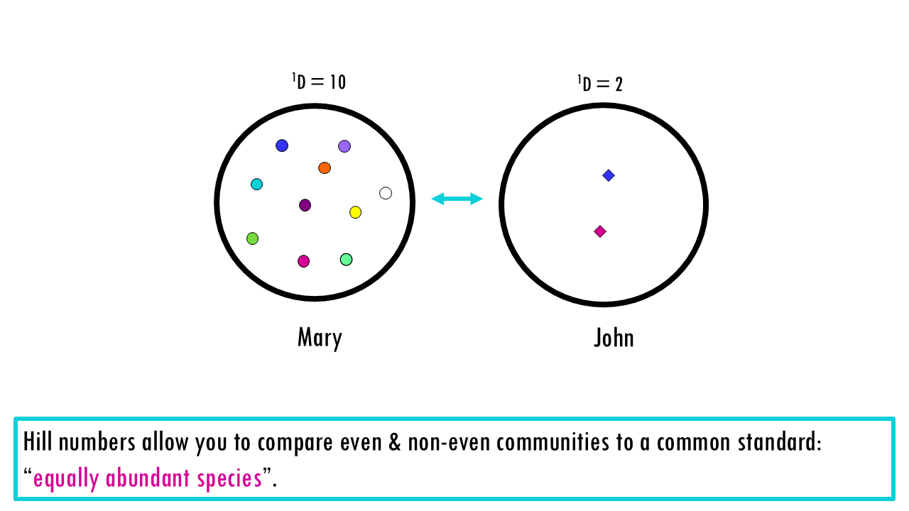
What’s great about transforming diversity to Hill numbers is that we can directly compare communities that are uneven, because we are using a common metric – “effective number of species in an even community”.

Even though John has 20 unique species or clonotypes, so his richness is higher than Mary’s, its Hill number tells you it is 5 times less diverse than Mary, or, in other words, Mary has five times as many effective species. The “linear” comparison works because you are comparing everything to a common standard: the Equally Abundant Species.

Nice! So now that we know that Hill numbers make diversity values between communities much more interpretable, which one do we use? D at q = 0, or 1, or 2?

Diversity profiles

Sometimes, we would like to compare the diversity of communities across all definitions of diversity: from taking into account only richness, to taking into account evenness. Remember each index (or corresponding Hill number!) takes more or less into account richness and evenness:

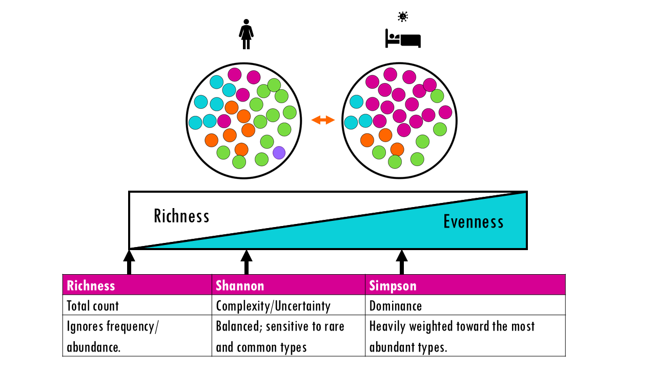
Rather than looking at a single number, Hill numbers allow you to see a diversity profile.

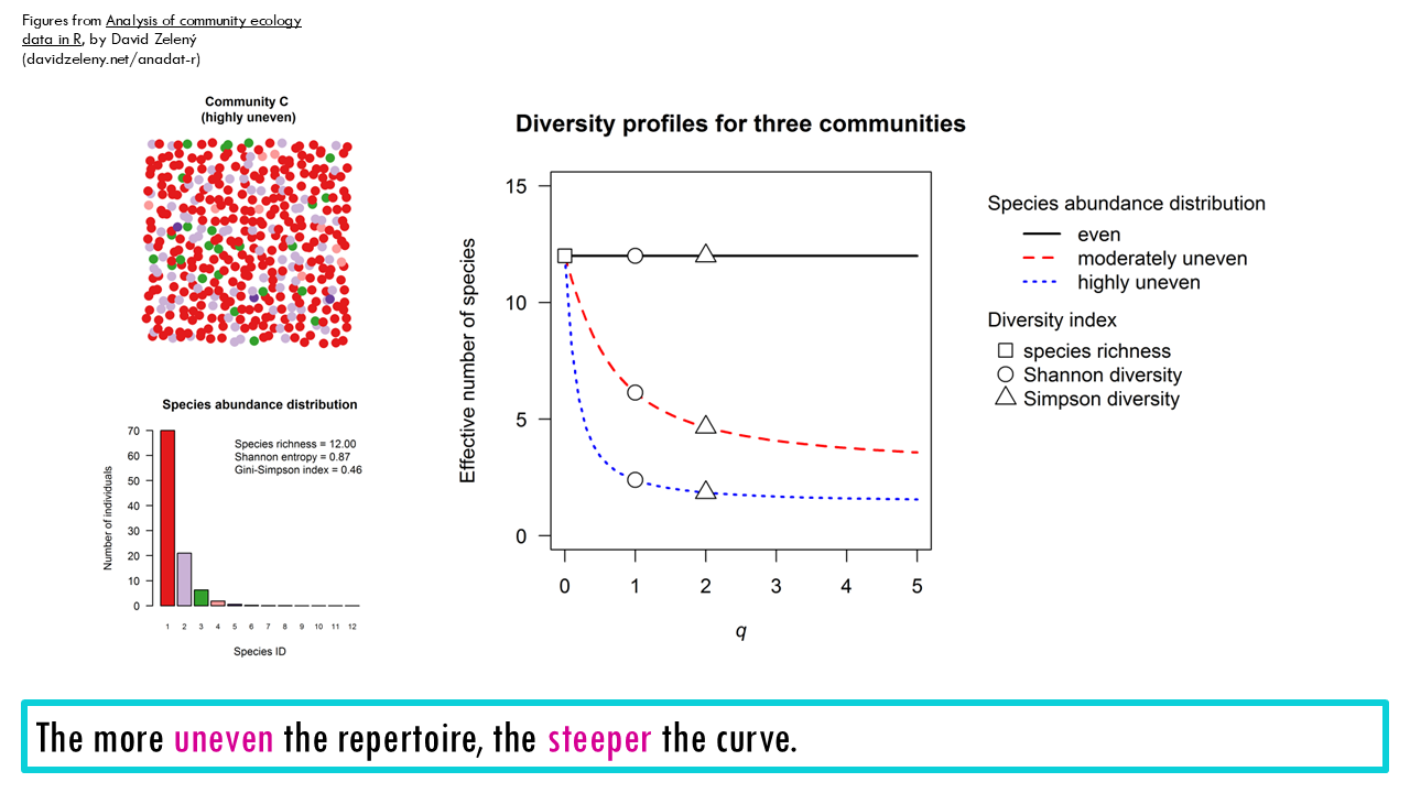
We’ve focused on three specific values of q, but by plotting ^qD against q (usually from q = 0 to q = 3) you get a Diversity Profile.

• Flat Curve: Suggests an even community (e.g., a healthy naïve B-cell pool where all clones have similar frequencies).
• Steeply Dropping Curve: Suggests an uneven repertoire. For example, after a viral infection, the richness (or effective number at q = 0) might remain high, but the effective number at q = 2, will be very low because a few clones have expanded massively and dominate the immune response.

Do you remember our example in our previous blogpost? We had 3 different communities, with A being perfectly even, B being moderately uneven and C being very uneven with 1 or 2 highly dominant species.

A diversity profile for A, B and C would look like this:

What if we had pre and post-infection samples? Would you be able to say which belongs to which curve? The blue curve corresponds to the pre-infection repertoire, whilst the pink steep curve is that of a more uneven repertoire.

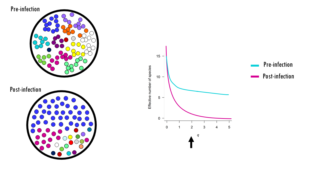
Note that in this example, the richness doesn’t change much. Sure, during infection a few more clones producing antibodies against the virus emerged, so the richness increased slightly. But take a look at q=1, which again, relates to Shannon Entropy. This is a more balanced view and often used to detect the shaping of the repertoire. Since a few clones started to expand during an infection, ¹D will drop significantly compared to ⁰D. If we want to give even more weight to dominant clones for the comparison of healthy versus infected, we can move onto the inverse Simpson index at q = 2 to measure the “effective number” of dominant clones. The low ²D suggests a highly polarized repertoire where a few massive clones dominate the population. It is very robust against sequencing errors because singletons have almost no impact on the value.

Final notes

Squidtastic!

In this blogpost we covered Hill numbers and how to interpret them. In essence, they are a unified family of diversity indices defined as the effective number of species, measuring biodiversity by combining species richness, Shannon diversity, and Simpson diversity into a single formula. They weight species based on abundance, providing a more intuitive, interpretable measure that solves limitations of traditional, non-linear indices. 

Want to know more?

Additional resources

If you would like to know more about single-cell integration methods, check out:

• Roswell et al., “A conceptual guide to measuring species diversity” — Hill numbers & coverage (practical guidance). 
• Barwell, Isaac & Kunin (2015), “Measuring β‑diversity with abundance data” — evaluation and properties of β metrics. 
• Jost L., “Entropy and diversity” (Oikos, 2006) — why convert entropies to effective numbers; Hill numbers & replication property. 
• Carpentries / metagenomics alpha–beta R tutorial — short instructional material and plotting examples. 

You might be interested in…

• UMAPs simply explained
• PCA simply explained
• t-SNE simply explained

Squidtastic!

Wohoo! You made it 'til the end!

Hope you found this post useful. If you have any questions, or if there are any more topics you would like to see here, leave me a comment down below. Your feedback is really appreciated and it helps me create more useful content:)

Otherwise, have a very nice day and... see you in the next one!

Before you go, you might want to check:

Squids don't care much for coffee,

but Laura loves a hot cup in the morning!

If you like my content, you might consider buying me a coffee.

You can also leave a comment or a 'like' in my posts or Youtube channel, knowing that they're helpful really motivates me to keep going:)

Cheers and have a 'squidtastic' day!