Understanding the structure of Seurat objects version 5 – step-by-step simple explanation!
If you’ve worked with single-cell RNAseq data, you’ve probably heard about Seurat. In this blogpost, we’ll cover the the Seurat object structure,in particular the new Seurat version 5. You can also follow the R tutorial here.
So if you are ready… let’s dive in!
Click on the video to follow my simple explanation on Seurat objects in R!
Seurat structure overview
Seurat is an R toolkit for single cell genomics. You can read more about it in the Satija lab main page.
When you work with single-cell data in R using the Seurat package, you’ll be working with a Seurat object. What does this mean?
First, let’s talk about what we mean by “single-cell data” and why we need a special type of data structure and not just a “regular ol’ dataframe”.
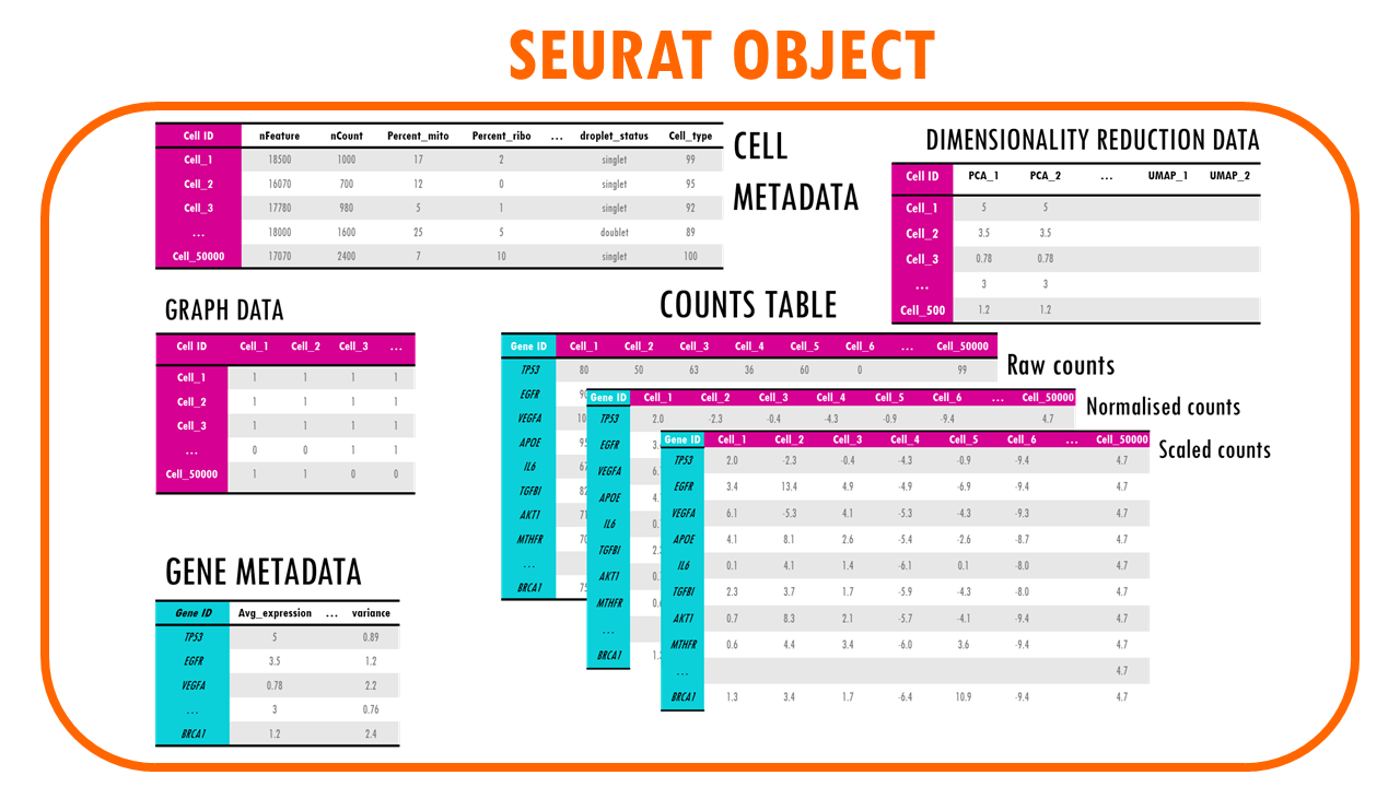
If we talk about single cell RNA seq data, we’re essentially talking about a table of counts. The rows are genes, and the columns are cells. We can then have metadata, which are annotations about the cells or the genes. And then we can have more complex data like reductions such as PCA, UMAP or tSNE which reduce the complexity of our dataset to lower dimensions, neighbours… The counts can be also have transformations, sometimes we need to work with raw counts, normalised counts, scaled counts…
This is why we need specific types of objects when we code to store all this data efficiently. Examples are anndata objects if you work in python, SummarisedExperiment or Seurat objects in R.
Seurat object: the “assay” slot
The Seurat object is a representation of single-cell expression data for R. Each Seurat object revolves around a set of cells and consists of one or more assay objects.
The assays have single-cell level expression data (whether that is RNA-seq, ATAC-seq, protein etc). If you are working with single-cell RNAseq data, then the assay will generally be “RNA”, which is the assay we’re going to be focusing on in this blogpost.
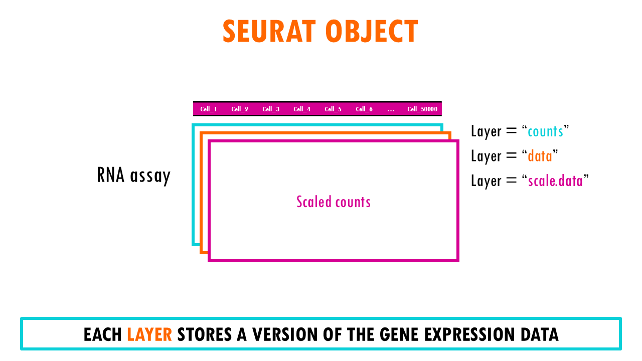
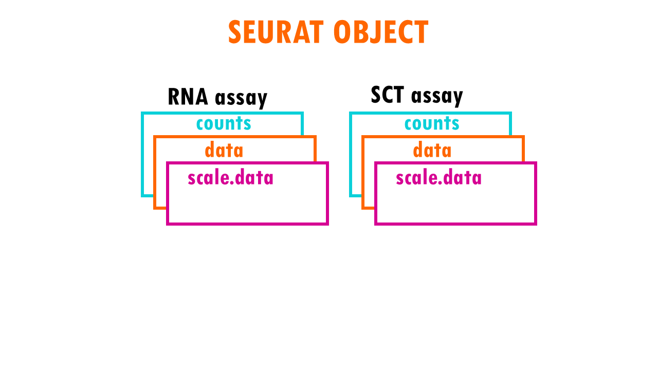
Each assay can have several layers. For example, when we first take our scRNAseq sequencing data and create our Seurat object, we will have the create the layer “counts” in the assay “RNA”. Counts is the layer for raw data. But as you very well know, in scRNAseq analysis we often used normalised counts or scaled counts, or batch-corrected counts to compare counts across cells, genes or samples / conditions. These different versions of the raw counts are stored in layers of our Seurat object.
The “data” layer
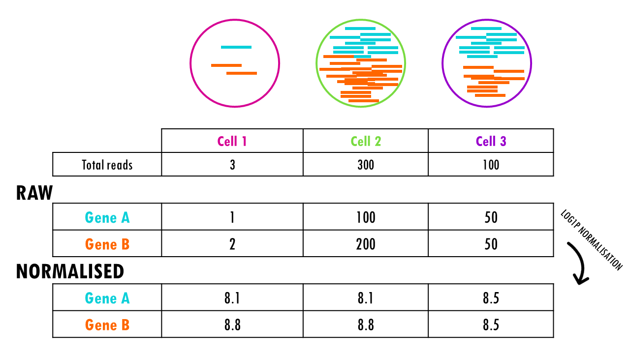
One of the key steps in data preprocessing involves normalising our data. Normalization is the process of adjusting the raw read counts to account for differences in sequencing depth (i.e., the total number of reads per cell) and other technical factors, ensuring that the expression levels are comparable across all cells. This is important because in scRNA-seq different cells often have different numbers of reads due to various factors like cell size, sequencing efficiency, or differences in the amount of RNA present in each cell.
So for example, if we wanted to compare the expression of Gene B in cells 1 and 2, it would seem like the expression of Gene B is 100 times higher in cell 2 compared to cell 1. But if we check the total number of reads, there were many more reads to begin with in cell 2. We need to correct for this, and that is what normalisation does.
In Seurat, by default, the function NormalizeData normalises raw counts using natural log (base e). Essentially, it:
- Divides each gene count by the total counts in that cell (in other words, the library size)
- Multiplies by a scale factor (default 10,000)
- Takes the natural logarithm (ln) and adds 1:
ln(normalized_value + 1).The function in R that does this is log1p.
Normalisation will make the reads comparable across cells. So now we see that the normalised counts for gene B are the same between cell 1 and cell 2, since both cells have double the number of counts for gene 2 compared to gene 1.
The normalised data in the Seurat object is stored in the layer “data”.
Squidtip
Normalization: This step addresses differences between cells by adjusting for sequencing depth or other technical variations, ensuring that gene expression values are comparable across cells.
The “scale.data” layer
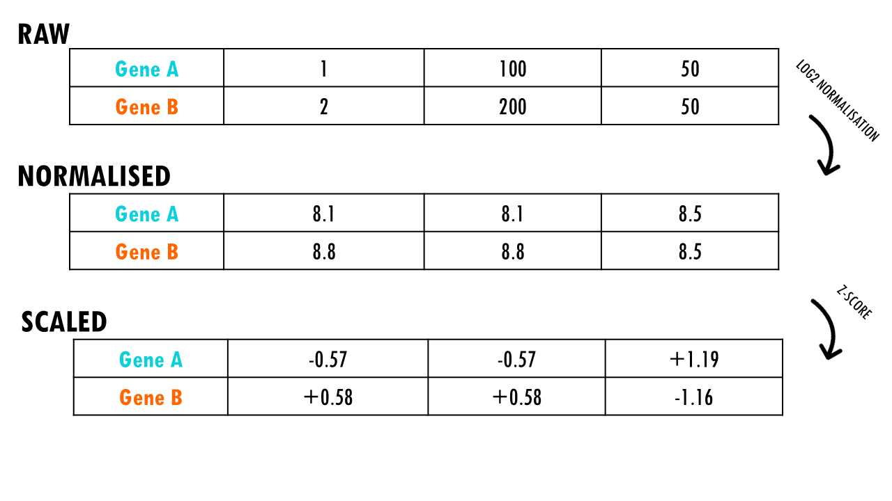
The second key step in data preprocessing is scaling. Scaling adjusts the expression values for each gene so that the expression values across cells are centered and comparable. It is particularly important in analyses like clustering or dimensionality reduction, where you want to ensure that all genes contribute equally to the analysis, rather than being biased by genes with inherently higher expression levels.
Z-scaling means that, for each gene, we subtract the mean expression of that gene across all cells and divide by the standard deviation. This results in a scaled expression value that has a mean of 0 and a standard deviation of 1 across all cells. This process makes the data centered and scaled, so each gene will contribute equally to the analysis.
The scaled data is stored in the layer “scale.data”.
Squidtip
Scaling: This step addresses differences between genes by adjusting for varying ranges in expression levels across genes, making sure that no single gene with very high expression dominates the analysis.
SCTransform: assay “SCT”
If you are used to working with Seurat objects, you might have already heard of SCTransform. SCTransform is an advanced normalization and transformation method specifically designed for single-cell RNA sequencing data. It is an alternative to traditional methods like log-normalization and scaling. The sctransform method uses a statistical model (regularized negative binomial regression) to perform normalization, accounting for both technical noise and biological variation in a more sophisticated way than simpler normalization techniques.
If you are interested in reading more about how sctransform actually works, check out my blogpost on sctransform. You can also check Seurat’s vignette on the SCTransform workflow here.
When we run sctransform on our data, a new “assay” will be created, the SCT assay. Again, you can expect the layers:
- counts, which has “transformed” or corrected raw counts
- data, the log-normalised versions of these corrected counts
- data, which has the Pearson residuals.
Squidtip
Sctransform is an advanced normalization and transformation method specifically designed for single-cell RNA sequencing (scRNA-seq) data. It is an alternative to traditional methods like log-normalization and scaling. The method is implemented in the Seurat package and uses a statistical model to perform normalization, accounting for both technical noise and biological variation in a more sophisticated way than simpler normalization techniques.
Seurat object: the “meta.data” slot
What other information can we store in a Seurat object?
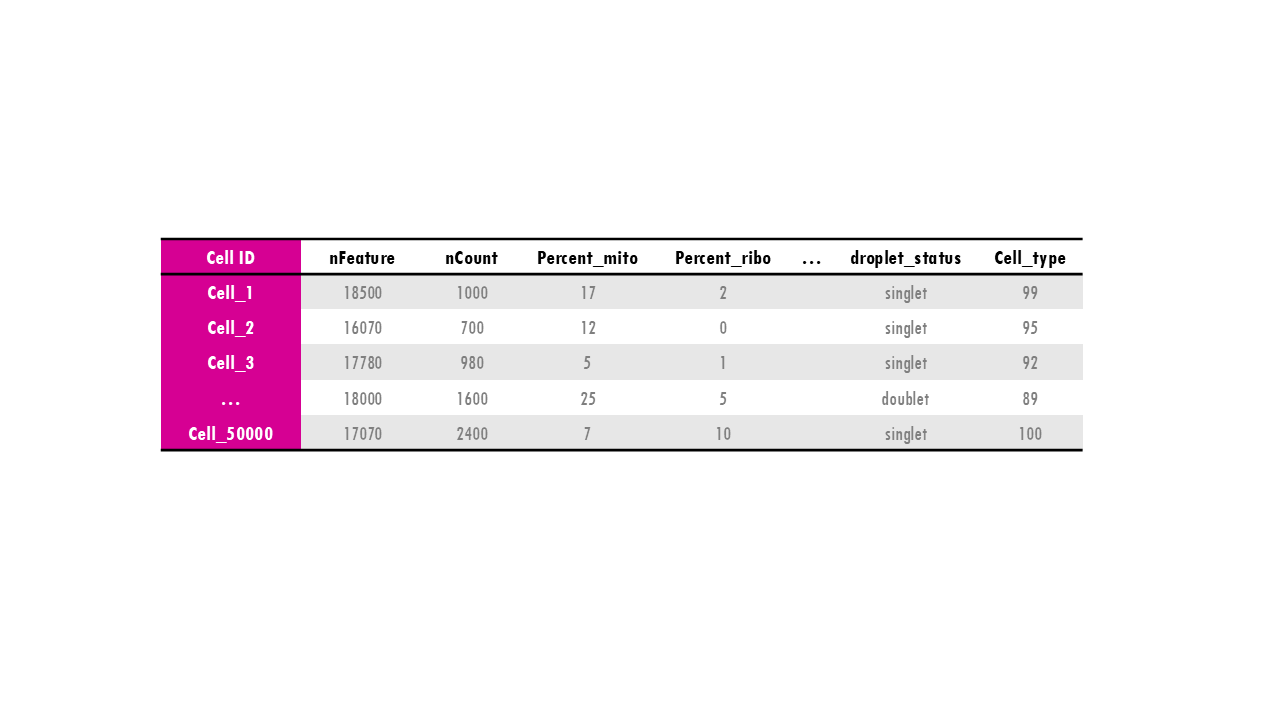
Of course, a very useful slot is the metadata slot. The metadata is used to store information about the cells: whether that is their cell type, their % of mitochondrial counts, whether they were treated or not during an experiment… This enables us, for example, to subset the Seurat object by a particular trait or to remove cells with a particular characteristic, or do differential expression between cells of different cell types. The metadata is just a dataframe with the cell IDs as rows and then different columns with metadata information. Easy!
Seurat object: the “reductions” slot
While processing our single cell data, we often want to visualise our cells. Common dimensionality reduction techniques are PCA, UMAP and t-SNE. We’ll talk about how to actually do this in my blogpost on Seurat workflow, but for now, know that all our dimensionality reduction results will be stored in the slot “reductions”. Examples are pca, tsne or umap. Each reduction stores a dimensionality reduction object, which contains information about the reduced coordinates (e.g., UMAP coordinates) and additional metadata like the variance explained by principal components.
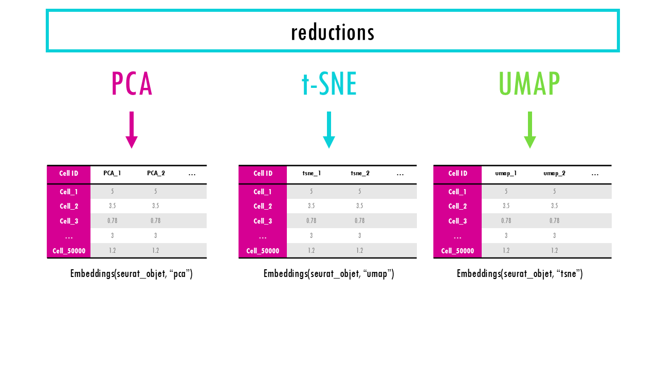
There are two main elements you need to know about.
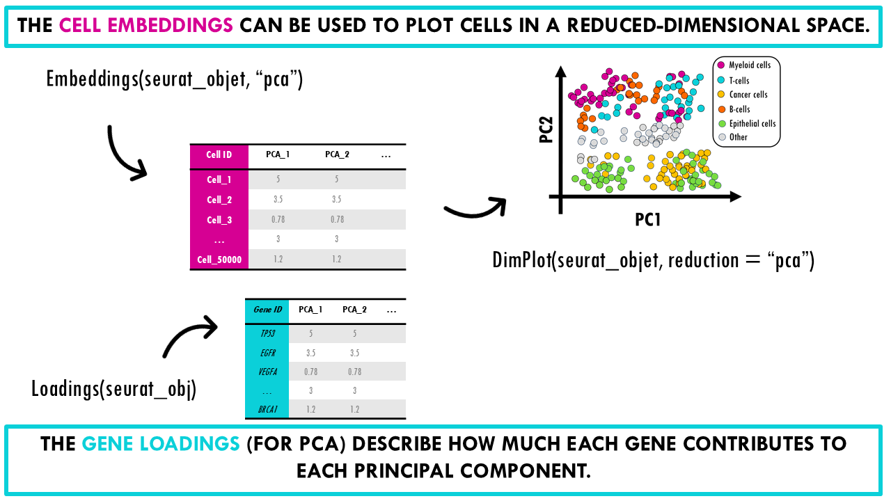
The first is the matrix of cell embeddings, which has the coordinates of each cell in a low-dimensional space that summarize the most important variation in the data; for that particular reduction method (i.e., PCA, UMAP, t-SNE…). You can access the embeddings with the function Embeddings(). This is the matrix used by DimPlot() when we want to plot a UMAP plot of our cells, for example. It’s essentially accessing the cell coordinates for UMAP_1 and UMAP_2. The embeddings are also used for visualization, clustering, batch correction, trajectory analysis, neighborhood graph construction, distance computations…
The second is the gene loadings in PCA, which describe how much each gene contributes to each principal component. They tell you which genes drive the variation captured by a given PC. You can access them with the function Loadings().
If embeddings describe cells in PC space, then loadings describe genes in PC space.
Squidtip
If you’d like to know more about dimensionality reduction methods and the differences between PCA, UMAP and t-SNE, check out this other blogpost!
Seurat object: the “graphs” slot
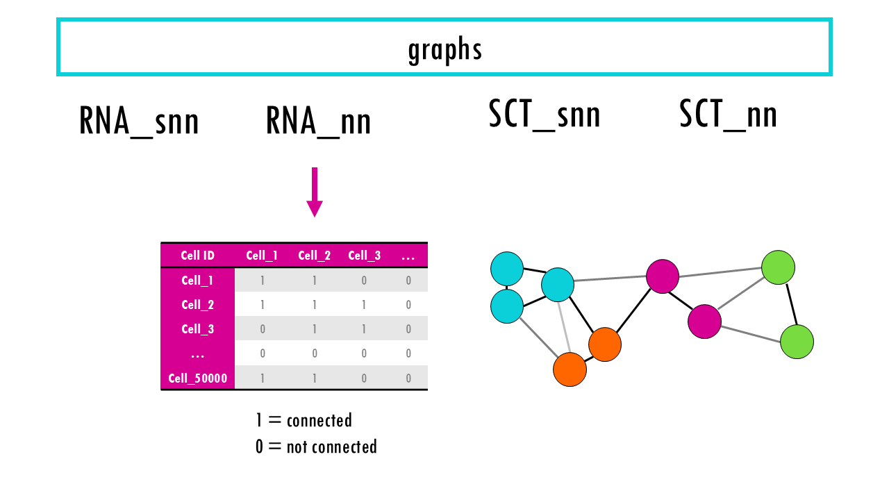
Finally, the graphs slot. It contains a list of graphs (usually a nearest-neighbor graph) that are used for clustering and other analyses. The graph typically represents relationships between cells based on gene expression similarity. For example, RNA_snn (a shared nearest-neighbor graph for RNA-seq data), or SCT_snn. We will talk a bit more about these graphs when we compute them!
Seurat structure: “commands” and “misc” slots
Finally, we’ll quickly mention the slots commands and misc.
Commands contains a record of the commands used to generate the object. This can help in reproducibility by storing a log of the methods and operations that were applied to create or manipulate the Seurat object.
And misc, for miscellaneous, is used to store arbitrary information that doesn’t fit into the other slots. It can be used to store additional analysis results or custom annotations.
Final notes
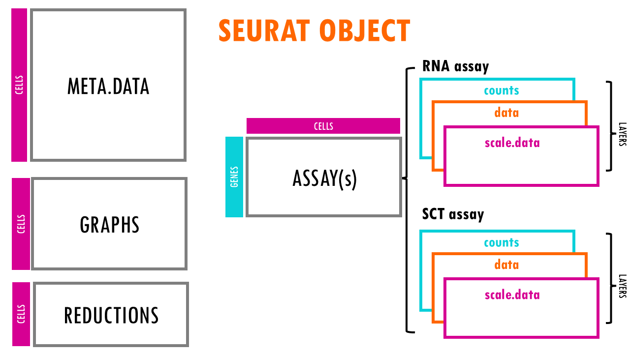
In a nutshell, a Seurat object is an R S4 object which allows us to store single-cell data in R.
The key slots in a Seurat object are:
- assays: This slot stores the raw and processed data in different forms. It is a list of Assay objects, each representing a specific type of data.
- Examples:
- RNA: The most commonly used assay, containing the raw and processed RNA counts.
- SCT: Stores data processed using SCTransform (a normalization method).
- integrated: Contains integrated data when datasets have been merged.
- Each assay can contain matrices like counts, data, and scale.data.
- Examples:
- meta.data:
- A data.frame containing metadata associated with each cell. This can include cell type annotations, experimental conditions, or other variables related to the cells.
- Example columns: cell_type, batch, condition, cluster.
- reductions:
- A list of dimensionality reductions applied to the data. These are used for visualizations like PCA, t-SNE, or UMAP.
- Examples: pca, tsne, umap.
- Each reduction stores a dimensionality reduction object, which contains information about the reduced coordinates (e.g., UMAP coordinates) and additional metadata like the variance explained by principal components.
- graphs:
- A list of graphs (usually a nearest-neighbor graph) that are used for clustering and other analyses. The graph typically represents relationships between cells based on gene expression similarity.
- Examples: RNA_snn (a shared nearest-neighbor graph for RNA-seq data), pca_snn.
- clusters:
- This stores the cluster assignments for each cell after a clustering analysis (e.g., Louvain or Leiden clustering). It is typically stored in the meta.data slot but can also be stored in a separate slot.
- commands:
- A record of the commands used to generate the object. This can help in reproducibility by storing a log of the methods and operations that were applied to create or manipulate the Seurat object.
- misc:
- This slot is used to store arbitrary information that doesn’t fit into the other slots. It can be used to store additional analysis results or custom annotations.
Want to know more?
Additional resources
If you would like to know more about Seurat objects, check out:
You might be interested in…
Ending notes
Wohoo! You made it ’til the end!
In this post, I shared some insights into the Seurat object structure.
Hopefully you found some of my notes and resources useful! Don’t hesitate to leave a comment if there is anything unclear, that you would like explained further, or if you’re looking for more resources on biostatistics! Your feedback is really appreciated and it helps me create more useful content:)
Before you go, you might want to check:
Squidtastic!
You made it till the end! Hope you found this post useful.
If you have any questions, or if there are any more topics you would like to see here, leave me a comment down below.
Otherwise, have a very nice day and… see you in the next one!
Squids don't care much for coffee,
but Laura loves a hot cup in the morning!

If you like my content, you might consider buying me a coffee.
You can also leave a comment or a 'like' in my posts or Youtube channel, knowing that they're helpful really motivates me to keep going:)
Cheers and have a 'squidtastic' day!


Hey,
Fantastic blog and was extremely helpful. However, are the values in the normalized gene expression in the middle columns correct? As they the raw counts of gene B is 2x gene A and after normalization they have the same value.
Best wishes,
Lukasz
Thank you so much for your feedback! That is a really good question – to give you a short answer (hoping to have time for a proper blogpost on this!) it happens because both genes maintained the same relative expression levels. Cell 2 was sequenced 100x deeper than Cell 1 so we’re just observing technical differences in sequencing depth. Essentially gene A remains 33.33% in both cells, and gene B is also 66.67% in both cells. So when we correct for library size and log-normalise, log normalisation essentially:
1. Normalises the values per cell (eliminating per-cell scale).
2. Log-transforms, compressing the fold changes.
So we can end up with the same value
However you are right in pointing out that the values should be different for each gene – I believe the correct values are 8.11 for Gene A (cell 1 and cell 2) and 8.81 for gene B (cell 1 and cell 2)
If you compute total counts per cell (library size) and scale by 10000, then take natural log, you should get something like:
| Gene | Cell 1 | Cell 2 | Cell 3 |
| —- | ———————- | ———————- | ——————- |
| A | ln(3334.33) ≈ **8.11** | ln(3334.33) ≈ **8.11** | ln(5001) ≈ **8.52** |
| B | ln(6667.67) ≈ **8.81** | ln(6667.67) ≈ **8.81** | ln(5001) ≈ **8.52** |
Hey, fantastic answer. Thank you for the correction. I would have just 2 wishes: could you write the equation on how to compute these values exactly in your blog (i.e. Gene A, Cell 1 = log2( Raw / Total * 10000 +1; I hope this is right), and correct the nice tables you have them, so there is no more error! Thanks for the amazing job!
Cheers,
Łukasz
Upon editing it, I realised Seurat’s default is the natural logarithm (https://satijalab.org/seurat/reference/normalizedata) so I just updated it with those values. Thanks again!
And yes, that’s right – just change ln instead of log2 if you want to do it with Seurat’s defaults.
Hey! Fantastic question- you inspired me to write a blogpost about it: https://biostatsquid.com/choose-thresholds-for-dge-analysis/
Hope it helps!
Thank you very much for this article! There is definitely a lack of documentation when it comes to the Seurat object structure.
What is the difference between the misc and tools slot? From what I could gather, the difference is that the tools slot is retained when performing operations like subsetting the object while the misc slot is dropped. Am I correct?
Also, it would be nice if you could add something about the images slot used for spatial data. I found quite challenging working with it as there is very little documentation available.
Hi! Thanks so much for your comment.
The tools slot typically contains outputs from functions like dimensional reduction results (e.g., from RunUMAP()), differential expression analysis, or other computational analyses – it’s generally reserved for tool developers to store internal data related to their specific methods. The misc slot is more for user-defined data, experimental metadata, or any additional information that doesn’t fit elsewhere; so you should use @misc if you have custom data you want to save. I’ve never had to use either to be honest, but the documentation here might help:https://github.com/satijalab/seurat/wiki/seurat
And thanks so much, that’s a fantastic suggestion – I’m hoping to do some spatial blogposts soon, so I’ll definitely take this into account!